CHAPTER FOURTEEN
Pricing Credit Risk
What should you get paid for taking a credit risk? The answer can be determined from an arbitrage between risk free (US Treasuries) and risky (corporate bonds) assets. For example, if, after all credit defaults, delays, and expenses, a diversified portfolio of 10-year corporates always returned more than a 10-year Treasury, rational investors would always buy the diversified corporate bond portfolio. However, if the Treasury always yielded more, rational investors would only buy Treasuries. In order for investors to buy both corporates and Treasuries, half the investors have to be convinced that the corporate portfolio will outperform and the other half are convinced that the Treasuries will outperform, otherwise there is an arbitrage situation.
Of course, the level of credit risk in the corporate portfolio is always changing due to changing macro- and microeconomic factors. So, if the two portfolios offer the same net return today, but credit risk increases, the Treasury will be more attractive. If credit risk declines, the corporate portfolio will be more attractive. Naturally, investors often disagree about whether credit risk is increasing or decreasing—which makes a market a market.
Suppose a 5% 1-year AAA eurobond is priced at $1,000. If an investor thought a 1-year CCC rated eurobond had a 10% chance of default and, in the event of default, zero recovery, what would it have to yield to fairly compensate the investor for the credit risk, if it too was priced at $1,000?
ANSWER:
If the risk free investment grows $1,000 to $1,050 in a year, the risky investment has to do the same. Thus:
(The probability of default × default return) + (The probability of survival × survival return) = $,1050
(10% × $0) + (90% × $X) = $1,050
$1,050 / .9 = $1,166.67
Return = 16.67%
If the CCC rated note was yielding more than 16.67%, the investor should buy the corporate note—if it was yielding less, the investor should buy the risk-free alternative. If instead the recovery was 30%, the yield would have to be:
(10% × $300) + (90% × $X) = $1,050
$1,020 / .9 = $1,133.33
Return = 13.33%
PROBLEM 14B
Let’s now look at a multiperiod example using a 3-year 10% eurobond priced at par. We assume default will only occur on an interest payment date since that’s the only time the company has payments due. Suppose an investor thought the data depicted in Figure 14.1 would apply.
FIGURE 14.1
Determining Fair Compensation for Credit Risk Over Multiple Periods
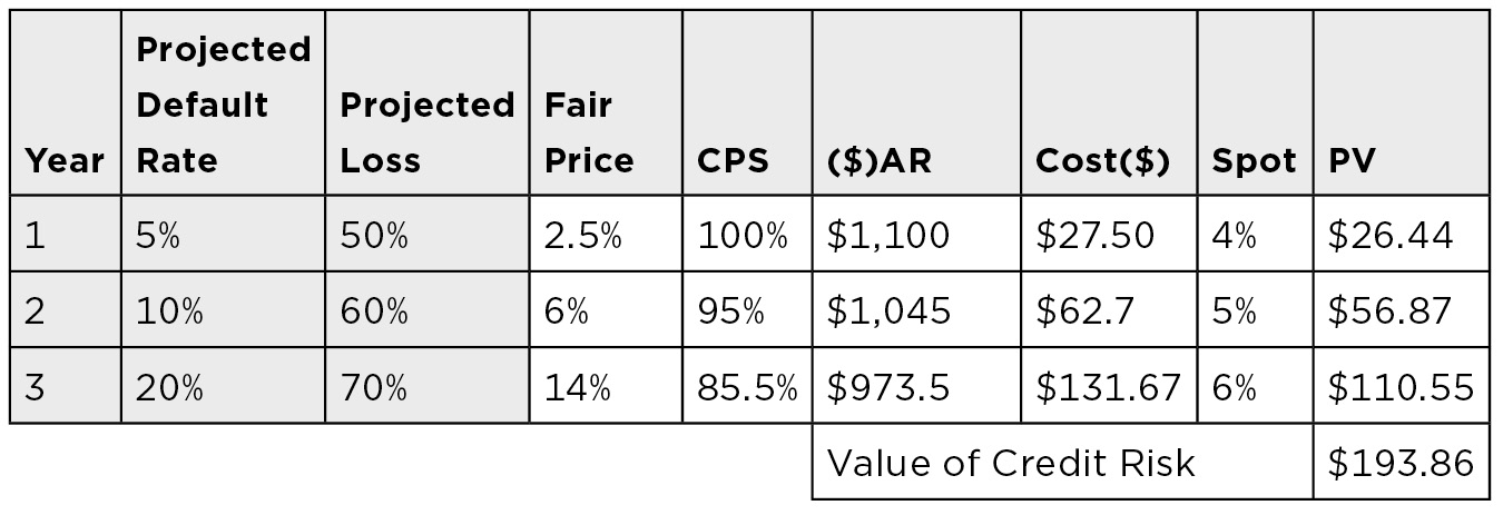
The fair price of credit risk is determined by multiplying the projected default rate by the projected loss in the event of default (Column 2 × Column 3). The conditional probability of survival (CPS) is the probability that the bond will still exist (that is, will not have defaulted) on the interest payment date, with the following:
- There is 100% probability the bond will make it to year 1 payment date.
- There is only a 95% probability the bond will make it to year 2 payment date. There is a 5% chance bond defaulted in year 1, so there is only a 95% chance the investor will need compensation for credit risk in year 2.
- There is only an 85.5% probability the bond will make it to year 3 interest payment date. There is 10% of a 95% chance (9.5%) the bond will default in year 2, so there is only an 85.5% chance the investor will need compensation for credit risk in year 3.
The annual amount at risk (($)AR) is ($1,000 principal + $100 interest) × CPS, which allows for previous defaults. The cost of credit protection paid on the interest payment date is determined by multiplying fair price by the annual amount at risk (Column 4 × Column 6). The spot rate from today to the interest payment date is shown in Column 8, and the PV of the cost of annual credit protection is shown in Column 9.
ANSWER:
The sum of Column 9 ($193.86) is the cost of buying a 3-year option that would protect the investor against default risk for 3 years. In the event of default:
- The investor would receive $1,100.
- The option seller would receive the note and would work through the bankruptcy process to recoup as much as possible.
Very often, protection buyers would rather pay for protection over time in a series of equal payments. Also, upon default, they want the payments to stop. In this case, we need to work backwards to determine the correct annual premium. The three premiums, when multiplied by the CPS and then discounted at the spot rates must total to $193.86—the cost of the option. Figure 14.2 illustrates the process.
Determining the Annual Credit Spread

DETERMINING PROBABILITY OF DEFAULT FROM CREDIT SPREAD
If we can use the probability of default and percentage recovery to determine the correct spread, we should also be able to work backwards in order to determine the implied probability of default from the expected recovery and the spread.
If we accept the arbitrage relationship between Treasuries and corporates, invest $1 in Treasuries for 1 year (assuming continuous compounding and ignoring recovery), then the FV of that $1 invested in Treasuries can be determined using the following formula:
FV = PVert = $1PVer1 = which simplifies to: er
The FV of that same $1 invested in corporates for 1 year (again, assuming continuous compounding) can be determined using the following formula, where:
- D = Default probability (you only get paid when bond doesn’t default)
- s = Spread to Treasuries
- R = Recovery percentage
For $1 and 1 year this simplifies to:
FV =(1–D)e(r+s)
Thus, the arbitrage between Treasuries and Corporates is: ert = (1–D)e(r+s)t
Rearranging the above gives us D = 1 − e–st
Thus, if the spread is 100 basis points on a 1-year instrument, then:
D = 1 − e–.0100(1) = .995% or just under 1%
If we add a recovery, then the FV of the Corporate Bond would be:
FV = (1–D)PVe(r+s)t + D(R) e(r+s)t
This changes the probability of default to:
D = (1 − e–st) / (1 − R)
PROBLEM 14C
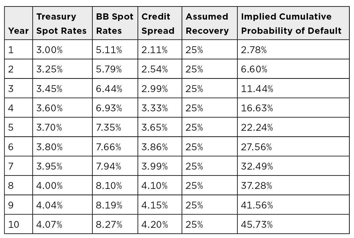
Use the information and formulas just presented and confirm the data found in Figure 14.3.
FIGURE 14.3
Confirm These Values
BANKRUPTCY AND BONDS
Despite the best efforts of management teams, sometimes companies can’t meet their current obligations and go bankrupt. The question then becomes, “What is a company that can’t meet its obligations worth?” The process for valuing a bankrupt company has two steps. Step one is to determine if, despite failing to meets its obligations, the company is a viable company. A viable company is defined as one whose “black box” generates positive cash flow. The black box is described in Figure 14.4.
FIGURE 14.4
Company’s Basic Black Box

A company buys raw materials, applies labor at its plant to create finished goods, sells the finished goods for cash, uses the cash to pay for the raw materials and labor, and hopefully has free cash left over. If it does, it may be a viable business. If the company doesn’t generate free cash, the business isn’t viable and will be liquidated.
Some businesses’ black boxes do generate significant free cash, but the free cash they generate is insufficient to cover one or more of the following:
- Service all the company’s debt obligations.
- Meet their promised employee benefit obligations (health care and/or pension obligations).
- Pay any and all legal judgments and liabilities.
This suggests that if those liabilities could be reduced, these companies and the jobs they offer could be saved. This is the role of the bankruptcy court judge. The court determines:
- First, if the company is viable.
- Second, if the company is viable, which liabilities need to be postponed, reduced, or canceled in order to allow the company to return to profitability.
To do this, the court must first value the company. The value of the company will be equal to a multiple of the free cash the company generates less the mandatory capital expenditures (CapX).
- The free cash approximately is what drops down from the black box.
- The CapX are the mandatory capital expenditures (such as replacing worn-out equipment) the company must make just to keep operating at its current level. Note that these CapX expenditures are not designed to grow the company either horizontally or vertically.
- The mandatory CapX are subtracted from the free cash.
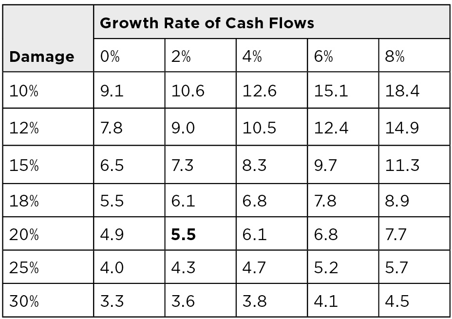
- The multiple applied to the remaining free cash flow is a function of the rate at which free cash is growing (or shrinking) and how damaged the business is by its having to file for bankruptcy. Figure 14.5 provides the approximate multiple for companies in bankruptcy.
FIGURE 14.5
Approximate Multipliers of (Free Cash − CapX) for Companies in Bankruptcy
Let’s look at an example.
PROBLEM 14D
Suppose a company has free cash flow of $250MM and has $30MM of mandatory capital expenses it must make to keep operating. Based on the company’s current condition and the rate at which its cash flow is growing, the multiple the judge uses is 6 times.
The company is valued at:
6 × (250MM − $30MM) = $1,320MM
With the value determined, we now turn to the company’s capital structure, which is illustrated Figure 14.6.
FIGURE 14.6
Example Company Capital Structure
|
Debt |
Amount |
|
Bank debt |
$220MM |
|
Senior unsecured debt |
$600MM |
|
Subordinated debt |
$750MM |
|
Junior subordinated debt |
$250MM |
The total debt load is $1,820MM, and the company is only worth $1,320MM. In other words, it currently has -$500MM of equity. Clearly, this is untenable. In this circumstance, the judge might elect to cancel both the subordinate debt and the junior subordinate debt. By canceling $1,000MM in debt, the company goes from having -$500MM of equity to having +$500MM of equity, as shown in Figure 14.7.
FIGURE 14.7
Debt Load Following Subordinate and Junior Subordinate Debt Cancellation
|
Debt |
Amount |
|
Bank debt |
$220MM |
|
Senior unsecured debt |
$600MM |
|
Subordinated debt |
$0MM |
|
Junior subordinated debt |
$0MM |
The $500MM of equity will be given to the subordinated debt holders, since they have the senior claim relative to the junior subordinated debt. So the new capital structure will be as shown in Figure 14.8.
FIGURE 14.8
Example Company New Capital Structure Following Equity Distribution
|
Debt |
Amount |
|
Bank debt |
$220MM |
|
Senior unsecured debt |
$600MM |
|
Equity |
$500MM |
In the bankruptcy, the:
- Bank debt is left on the company’s balance sheet.
- Senior unsecured debt is left on the company’s balance sheet.
- The subordinated debt holders lose $750MM of debt but receive $500MM of equity. In short, they get $2 of equity for every $3 of debt they owned—a 66% recovery.
- The junior subordinated debt holders receive no equity because there isn’t enough equity to make the debt level above them whole. They are wiped out, as are any lower levels in the capital structure.
Now, the interesting story of the above is the subordinated debt holders. As the company’s credit quality declines, the value of the subordinated debt declines. The original purchasers (banks, insurance companies, individuals) sell in order to limit their loss. The buyers of this deeply distressed debt are the private equity and hedge funds. Let’s suppose these secondary market buyers paid, on average, $0.50 on the $1 for the subordinated debt. Thus, the $750MM of subordinated debt cost them just $375MM.
In the bankruptcy, they exchange their bonds for $500MM worth of stock. So, they end up with 100% of the stock worth $500MM by losing bonds they bought for just $375MM—making $125MM in the bankruptcy process. They will hire a new management team to fix the company and grow it for a few years. Then, they will sell the company to a larger firm at a profit or take the company public. Every private equity manager will tell you that the best place to buy stock is not the floor of the New York Stock Exchange—but on the steps of the bankruptcy court.
When the various stakeholders agree on the value of the company and who should get what, they can go to the bankruptcy court with a prepackaged bankruptcy. In the example bankruptcy we just discussed:
- The bank is made whole, so it has no complaints.
- The senior bondholders are made whole with debt, so they have no complaints.
- The “current” subordinated debt holders made $125MM and ended up with 100% of the equity, so they are happy.
- The junior subordinated bondholders are unhappy but, even if the company was valued $150MM higher, they still wouldn’t be entitled to any recovery.