CHAPTER SIXTEEN
Active Portfolio Management
Investors who actively manage their portfolios try to outperform the market. They anticipate how the market will change and then position their portfolios to profit from that change. Active portfolio management usually requires additional trading, market data, analytics, and/or personnel, so the active strategy has to generate an extra return that exceeds these additional costs in order to provide real value added. Active strategies fall into two categories: Those that are designed to outperform an index and those that are designed to boost total return without regard to any index. Let’s start with strategies that are designed to outperform an index.
For this section the index we will use is the Barclays Aggregate Taxable Index. This index includes US Treasuries, US agencies, investment grade corporates, and insured mortgage-backed securities. Let’s assume it has the characteristics depicted in Figure 16.1.
Barclays Aggregate Data
|
Barclays Aggregate |
|
|
Weighted average coupon |
4.96% |
|
Weighted average maturity |
12.22 |
|
Weighted average yield |
3.96% |
|
Duration |
7.61 |
|
Modified duration |
7.40 |
|
Convexity |
21 |
|
Percent AAA |
72% |
|
Percent AA |
16% |
|
Percent A |
5% |
|
Percent BBB |
7% |
|
Percent Treasuries |
31% |
|
Percent agencies |
14% |
|
Percent corporates |
19% |
|
Percent mortgages |
36% |
There are three ways to outperform an index:
- Buy individual securities that mirror the index but are less liquid than the index.
- Buy four ETFs (Treasury, agency, MBS, corporates) held in percentages that mirror the index, and then make active reallocation bets.
- Buy three of the four ETFs, and actively manage the sector where the investor has a competitive advantage.
Let’s look at these three alternative methodologies in greater detail.
LIQUIDITY APPROACH
Less liquid securities offer a higher yield than otherwise identical securities that are more liquid. An 8% A rated 20-year bond from a small offering will offer a higher yield than an 8% A rated bond from a $1 billion offering. A $1MM 6% GNMA with a $115K remaining balance will trade at a higher yield than a $1 billion 6% GNMA with an $800MM remaining balance. To the extent an investor can duplicate the index with less liquid securities, the investor can slightly outperform. However, this strategy makes sense only for long-term investors.
FOUR ETF APPROACH
An investor who buys four ETFs that collectively mirror the index can easily make volatility bets by overweighting/underweighting asset classes. Depending on expectations, the investor should use the following courses of action:
- Interest rate volatility increases—The investor should underweight the MBS ETF that has negative convexity and overweight the UST ETF that has positive convexity. Reverse the trade if interest rate volatility is expected to decline.
- Credit spread declines—The investor should overweight the CORP ETF and underweight the UST ETF. Reverse the trade if credit spreads are expected to widen.
- Interest rate declines—The investor should sell 5% or 10% of the ETF shares and buy long-term bonds, long-term zeros, and Treasury zeros. The long-term bonds have durations higher than 7.61 and so will boost the duration of the overall portfolio. If rates decline, the investor’s portfolio will outperform. Stick with Treasuries to minimize transaction costs and maximize liquidity. After rates have declined, sell the Treasuries at a profit and repurchase shares in the ETF(s). Of course, if the investor expected rates to rise the investor should sell 5% to 10% of the ETF shares and invest in cash and/or floating rate notes that shorten the portfolio’s duration relative to the index. If rates do rise, the investor’s portfolio will suffer a smaller loss—and therefore outperform.
THREE ETF APPROACH
In this approach, the investor buys three of the four ETFs—but actively manages the fourth market sector. For example, if the investor has a real expertise in credit analysis, the investor should buy the MBS, AGCY, and UST ETFs and actively manage the corporate bond portfolio. If the investor’s skill allows them to outperform the corporate index and the investor ties the other three sectors, the portfolio as a whole will outperform.
TOTAL RETURN
An investor who is not competing against a benchmark is said to be seeking total return. They can implement all of the strategies we just discussed, as well as a few strategies unique to total return investors. The two most common ones are:
- Riding the yield curve
- Yield curve plays
Let’s look at them now.
Riding the Yield Curve
Suppose you want to invest $1MM for 1 year, and you have two choices:
- Bond A—Buy a 1-year $1,000 investment priced at par with a coupon of 5%.
- Bond B—Buy a 2-year $1,000 investment priced at par with a coupon of 6%, and sell it in a year.
If you expect the yield curve to remain unchanged over the next year, which is a better buy?
FIGURE 16.2
Initial Choice

As shown in Figure 16-3, if the yield curve remains unchanged, then in 1 year:
- Bond A matures at par and yields 5%.
- Bond B still has a year of life left, and so must be sold. However, over the next year, the 2-year note becomes a 1-year note. Thus, in 1 year, it’s a 1-year note with a 6% coupon and could be sold at a premium.
FIGURE 16.3
After a Year

If the 6% coupon note is sold as a 1-year note offering a 5% return, the net performance of the two notes is as shown in Figure 16.4.
FIGURE 16.4
Relative Performance of Two Notes If Rates Stay Constant
|
1-Year 5% |
2-Year 6% |
|
|
Buy |
5% |
6% |
|
Sell |
NA |
5% |
|
Income |
$50 |
$60 |
|
Gain |
$0 |
$9.52 |
|
Total |
$50 |
$69.52 |
The 2-year note earns $69.52, instead of $50.00, which is an incremental return of $19.52 or 39%. Of course, buying the 2-year note and selling it in 1 year is not a risk-free strategy. If interest rates rise, the value of the 2-year note can decline. For example, suppose over the next year interest rates rise by 1%, as shown in Figure 16.5.
FIGURE 16.5
Interest Rates Rise by 1%

In this case, the benefit of riding down the yield curve from 2 years to 1 year is offset by the yield curve rising by 1%, as described in Figure 16.6.
FIGURE 16.6
Relative Performance of Two Notes If Rates Rise by 1%
|
1-Year 5% |
2-Year 6% |
|
|
Buy |
5% |
6% |
|
Sell |
NA |
6% |
|
Income |
$50 |
$60 |
|
Gain |
$0 |
$0 |
|
Total |
$50 |
$60 |
If rates rise by 1%, the 2-year note still generates an extra $10—or a 20% incremental return. One-year rates in 1 year would have to rise to almost 7% before the return on the two notes is equal and above 7% before the 1-year note offers a higher return.
The steeper the yield curve, the greater the advantage of riding down the curve. Look at the curves shown in Figure 16.7.
FIGURE 16.7
Two Curves

- Along the lower curve, as time passes the yield declines by 1% over the first year and another 1% over the next 6 months.
- Along the higher curve, as time passes the yield declines by 2% over the first year and another 2% over the next 6 months. The larger the decline in rates, the greater the rise in price.
Figure 16.8 provides details about the pricing of the coupon bonds along both curves.
Price of Current Coupon Bond Along Both Curves
|
Start |
In 1 Year |
In 18 Months |
|
|
High Curve |
9%—$1,000 |
7%—$1,018.69 |
5%—$1,019.28 |
|
Low Curve |
6%—$1,000 |
5%—$1,009.52 |
4%—$1,009.71 |
As time passes, there are two offsetting factors that impact the price of the note. The decline in rates causes the price to rise. The passage of time causes a pull toward par at maturity. If you hold the note too long, the pull toward par exceeds the benefit of rates declining. As a general rule, sell about halfway to maturity. If you buy a 2-year note when the yield curve is steep, sell it in a year. If you buy a 3-year note, sell it in 18 months. Reinvest the proceeds where the curve starts to be steep and reap the profits.
MAKING YIELD CURVE BETS
Yield curve shifts are often nonparallel. Short-term rates can be rising while long-term rates are stable—or even declining. Fed actions that have immediate impact at the short end of the curve may:
- Have no impact at the long-term rates
- Only have an impact after a lengthy delay
- Cause long-term rates to move the opposite way
Likewise, inflation can cause long-term rates to rise over a multi-year time frame before the Fed chooses to react by raising short-term rates. At the intermediate point of the curve, mortgage activity may heat up—putting pressure on the 10-year point of the curve, without materially impacting the short end or the long end of the curve. For example, suppose an investor expects the Fed to drastically raise short-term rates in an effort to control inflation and, as a result, you expect the yield curve to invert as illustrated in Figure 16.9.
FIGURE 16.9
Current vs. Expected Yield Curve
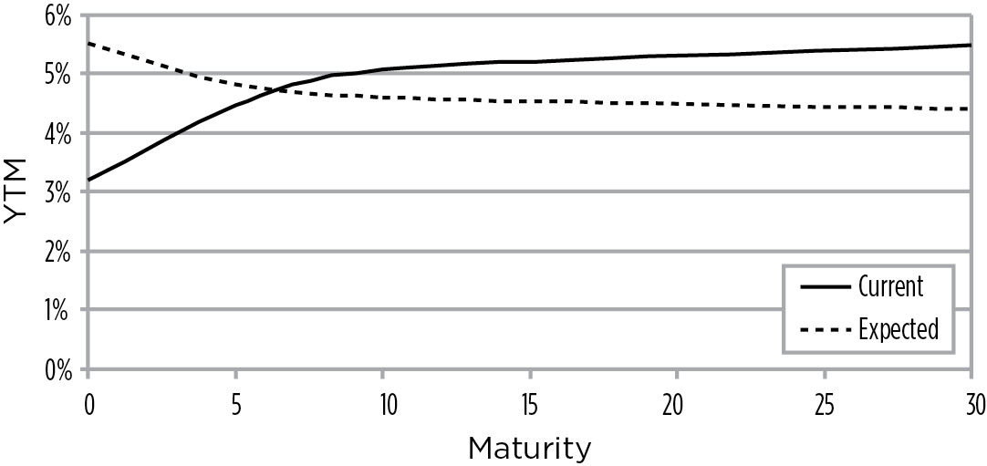
Given this outlook, you might want to go long 20-year euro ZCBs and short 1-year euro ZCBs. Assuming the 20-year ZCBs yields 6% and the 1-year ZCB yields 3%, the value of .01 ΔIR for each would be:
20-year = MV × MD × .0001
20-year = 1,000 / (1.06)20 × (20 / 1.06) × .0001
20-year = $311.80 × 18.87 × .0001
20-year = $0.588
1-year = MV × MD × .0001
1-year = 1,000 / 1.031 × 1 / 1.03 × .0001
1-year = $970.87 × .971 × .0001
1-year = $0.0945
Thus, the ratio of bonds that is necessary to have equal volatility on both sides is 6.24. In this case, you would go short 6.24 1-year ZCBs for each long 20-year ZCB. By having equal volatility, the investor is not exposed to parallel shifts in rates. If rates rise or fall in general, the gain and loss offset each other. This position profits from a yield curve flattening and loses if the yield curve steepens. Assume an investor went short $6.4 MM of 1-year ZCBs and long $1MM of the 20-year ZCBs. If short rates rise 150 basis points and long rates decline 20, the net profit would be approximately:
Short position = 6,400 bonds × 50 × $.0945 = $30,200
Long position = 1,000 bonds × 20 × $.588 = $11,760
There are numerous opportunities to put on yield curve plays during the typical economic cycle, as shown in Figure 16.10.
FIGURE 16.10
Start of the Business Cycle

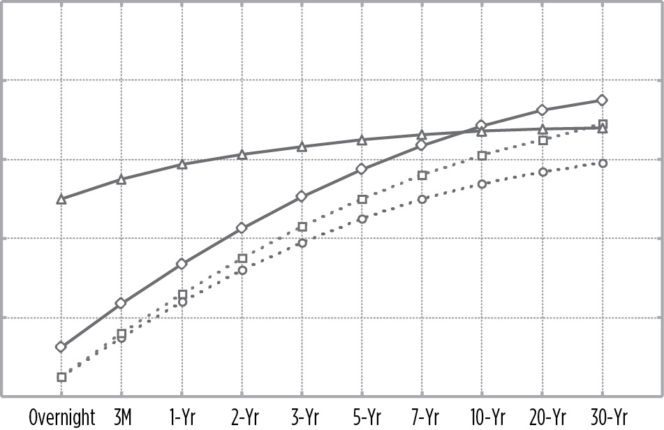
At the start of the business cycle, the yield curve normally has a positive slope, but it is fairly flat. As the economy heats up, inflation fears enter the economy, and long-term rates start to rise because long-term investors take more inflation risk, as depicted in Figure 16.11.
FIGURE 16.11
Long-Term Rates Rise

When long-term rates start to rise, the Fed tends to react slowly, so long-term and short-term rates start to rise in conjunction with long-term rates. This rise is parallel, as shown in Figure 16.12.
Parallel Rise

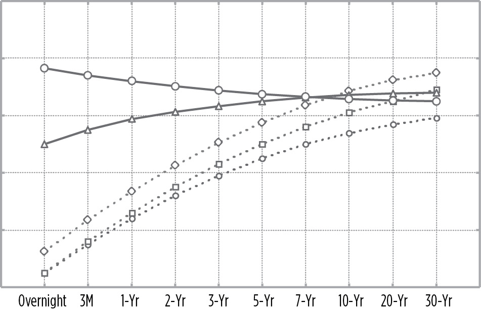
The Fed then gets serious about fighting inflation and raises short-term rates dramatically. This usually causes long-term rates to start declining, as shown in Figure 16.13.
FIGURE 16.13
Fed Dramatically Raises Short-Term Rates
Sometimes the Fed overreacts and raises short-term rates too far, which results in an inverted yield curve. As a result, long-term rates fall faster, as illustrated in Figure 16.14.
FIGURE 16.14
Inverted Yield Curve
After successfully pushing down long-term rates, the Fed can lower short-term rates (Figure 16.15).
Fed Lowering Rates After Success

Then the cycle starts over, as illustrated in Figure 16.16.
FIGURE 16.16
The Cycle Repeats

Some additional strategies that are beyond the scope of this text include:
- More than one currency—Global portfolios provide the opportunity to overweight bonds in currencies you expect to get stronger.
- Covered option writing—Selling out of the money options on bonds in the portfolio can allow you to generate additional revenue.
- Future credit quality—Predicting the future credit quality of individual bonds can also generate revenue.