© Orhan Gazi Yalçın 2021

O. G. YalçınApplied Neural Networks with TensorFlow 2https://doi.org/10.1007/978-1-4842-6513-0_7

7. Convolutional Neural Networks

Orhan Gazi Yalçın¹  

(1)

Istanbul, Turkey

 

It is safe to say that one of the most powerful supervised deep learning models is convolutional neural networks (abbreviated as CNN or ConvNet). CNN is a class of deep learning networks, mostly applied to image data. However, CNN structures can be used in a variety of real-world problems including, but not limited to, image recognition, natural language processing, video analysis, anomaly detection, drug discovery, health risk assessment, recommender systems, and time-series forecasting.

CNNs achieve a high level of accuracy by assembling complex patterns using the more basic patterns found in the training data. For instance, from lines to an eyebrow, from two eyebrows to a human face, and then to a full human figure, CNNs can correctly detect humans in an image by using mere lines. To assemble these patterns, CNNs require a small amount of data preparation since their algorithm automatically performs these operations. This characteristic of CNNs offers an advantage compared to the other models used for image processing.

Today, the overall architecture of the CNNs is already streamlined. The final part of CNNs is very similar to feedforward neural networks (RegularNets, multilayer perceptron), where there are fully connected layers of neurons with weights and biases. Just like in feedforward neural networks, there is a loss function (e.g., crossentropy, MSE), a number of activation functions, and an optimizer (e.g., SGD, Adam optimizer) in CNNs. Additionally, though, in CNNs, there are also Convolutional layers, Pooling layers, and Flatten layers.

In the next section, we will take a look at why using CNN for image processing is such a good idea.

Note

I will usually refer to image data to exemplify the CNN concepts. But, please note that these examples are still relevant for different types of data such as audio waves or stock prices.

Why Convolutional Neural Networks?

The main architectural characteristic of feedforward neural networks is the intralayer connectedness of all the neurons. For example, when we have grayscale images with 28 x 28 pixels, we end up having 784 (28 x 28 x 1) neurons in a layer that seems manageable. However, most images have way more pixels, and they are not in grayscale. Therefore, when we have a set of color images in 4K ultra HD, we end up with 26,542,080 (4096 x 2160 x 3) different neurons in the input layer that are connected to the neurons in the next layer, which is not manageable. Therefore, we can say that feedforward neural networks are not scalable for image classification. However, especially when it comes to images, there seems to be little correlation or relation between two individual pixels unless they are close to each other. This important discovery led to the idea of Convolutional layers and Pooling layers found in every CNN architecture.

CNN Architecture

Usually, in a CNN architecture, there are several convolutional layers and pooling layers at the beginning, which are mainly used to simplify the image data complexity and reduce their sizes. In addition, they are very useful to extract complex patterns from the basic patterns observed in images. After using several convolutional and pooling layers (supported with activation functions), we reshape our data from two-dimensional or three-dimensional arrays into a one-dimensional array with a Flatten layer. After the flatten layer, a set of fully connected layers take the flattened one-dimensional array as input and complete the classification or regression task. Let’s take a look at these layers individually.

Layers in a CNN

We are capable of using many different layers in a convolutional neural network. However, convolutional, pooling, and fully connected layers are the most important ones. Therefore, let’s quickly cover these layers before we implement them in our case studies.

Convolutional Layers

A convolutional layer is the very first layer where we extract features from the images in our datasets. Since pixels are only related to the adjacent and other close pixels, convolution allows us to preserve the relationship between different parts of an image. The task of a convolutional layer merely is filtering the image with a smaller pixel filter to decrease the size of the image without losing the relationship between pixels. When we apply convolution to a 5 x 5 pixel image by using a 3 x 3 pixel filter with a 1 x 1 stride (1-pixel shift at each step), we end up having a 3 x 3 pixel output (64% decrease in complexity) as shown in Figure 7-1.

Figure 7-1

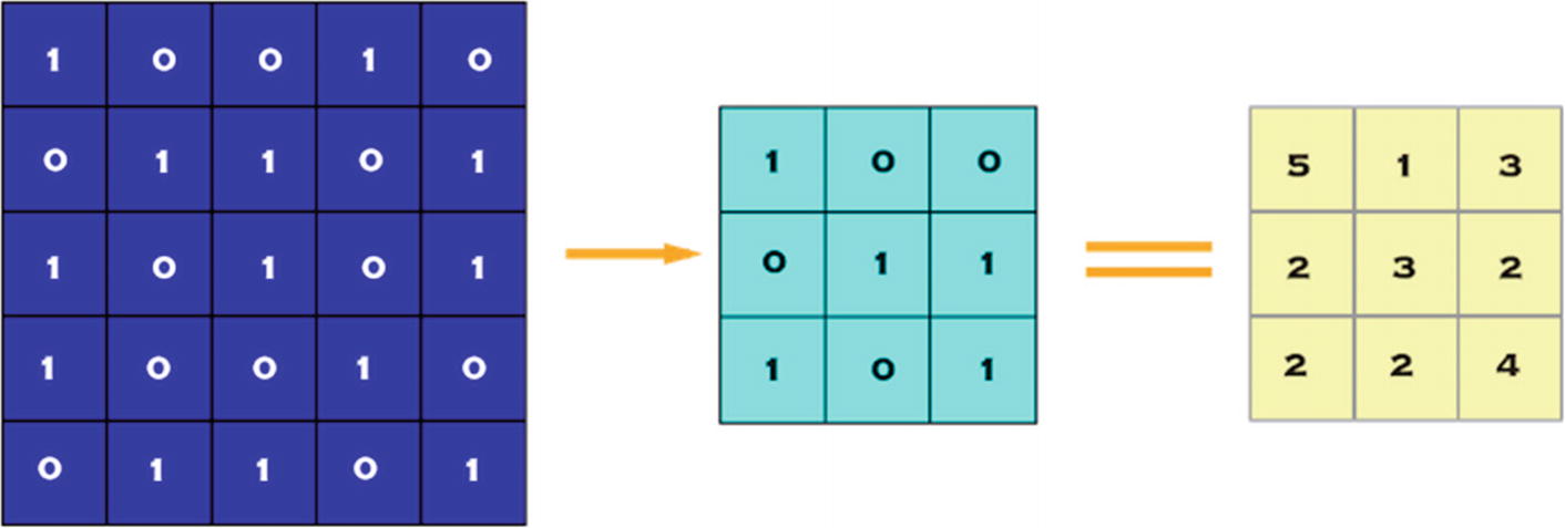
Convolution of 5 x 5 Pixel Image with 3 x 3 Pixel Filter (Stride = 1 x 1 pixel)

Filtering

Filtering is performed by multiplying each value in a part of the image data with the corresponding filter value. In Figure 7-2, the very first operation is as follows. (Please refer to Table 7-1 for all convolution operations shown in Figure 7-1).

Figure 7-2

The Very First Filtering Operation for the Convolution Shown in Figure 7-1

Table 7-1

The Table of Calculations for Figure 7-2

Rows	Calculations	Result
1st row	(1x0) + (0x0) + (0x0) +
2nd row	(0x0) + (1x1) + (1x1) +	= 5
3rd row	(1x1) + (0x0) + (1x1)

Using a too large filter would reduce the complexity more, but also cause the loss of important patterns. Therefore, we should set an optimal filter size to keep the patterns and adequately reduce the complexity of our data.

Strides

Stride is a parameter to set how many pixels will the filter shift after each operation. For the example earlier

• If we select a 1 x 1 pixel stride, we end up shifting the filter 9 times to process all the data.

• If we select a 2 x 2 pixel stride, we can process the entire 5 x 5 pixel image in 4 filter operations.

Using a large stride value would decrease the number of filter calculations. A large stride value would significantly reduce the complexity of the model, yet we might lose some of the patterns along the process. Therefore, we should always set an optimal stride value – not too large, not too small.

Pooling Layer

When constructing CNNs, it is almost standard practice to insert pooling layers after each convolutional layer to reduce the spatial size of the representation to reduce the parameter counts, which reduces the computational complexity. In addition, pooling layers also help with the overfitting problem.

For pooling operation, we select a pooling size to reduce the amount of the parameters by selecting the maximum, average, or sum values inside these pixels. Max pooling, one of the most common pooling techniques, may be demonstrated as follows.

Figure 7-3

Max Pooling by 2 x 2

In pooling layers , after setting a pooling size of N x N pixels, we divide the image data into N x N pixel portions to choose the maximum, average, or sum value of these divided portions.

For the example in Figure 7-3, we split our 4 x 4 pixel image into 2 x 2 pixel portions, which gives us 4 portions in total. Since we are using max pooling, we select the maximum value inside these portions and create a reduced image that still contains the patterns in the original image data.

Selecting an optimal value for N x N is also crucial to keep the patterns in the data while achieving an adequate level of complexity reduction.

A Set of Fully Connected Layers

Fully connected network in a CNN is an embedded feedforward neural network, where each neuron in a layer is linked to the neurons in the next layer to determine the true relation and effect of each parameter on the labels. Since our time-space complexity is vastly reduced thanks to convolution and pooling layers, we can construct a fully connected network at the end of our CNN to classify our images. A set of fully connected layers looks like as shown in Figure 7-4:

Figure 7-4

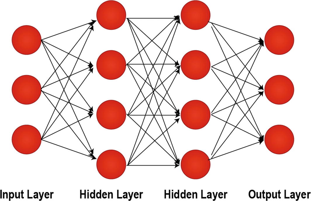
A Fully Connected Layer with Two Hidden Layers

A Full CNN Model

Now that you have some idea about the individual layers of CNNs, it is time to share an overview look of a complete convolutional neural network in Figure 7-5:

Figure 7-5

A Convolutional Neural Network Example

While the feature learning phase is performed with the help of convolution and pooling layers, classification is performed with the set of fully connected layers.

Case Study | Image Classification with MNIST

Now that we covered the basics of convolutional neural networks, we can build a CNN for image classification. For this case study, we use the most cliché dataset used for image classification: MNIST dataset, which stands for Modified National Institute of Standards and Technology database. It is an extensive database of handwritten digits that is commonly used for training various image processing systems.

Downloading the MNIST Data

The MNIST dataset is one of the most common datasets used for image classification and accessible from many different sources. Tensorflow allows us to import and download the MNIST dataset directly from its API. Therefore, we start with the following two lines to import TensorFlow and MNIST dataset under the Keras API.

import tensorflow as tf

import tensorflow_datasets as tfds

(x_train,y_train),(x_test,y_test)=tfds.as_numpy(tfds.load('mnist', #name of the dataset

        split=['train', 'test'], #both train & test sets

        batch_size=-1, #all data in single batch

        as_supervised=True, #only input and label

        shuffle_files=True #shuffle data to randomize

  ))

The MNIST database contains 60,000 training images and 10,000 testing images taken from American Census Bureau employees and American high school students. Therefore, in the second line, we separate these two groups as train and test and also separate the labels and the images. x_train and x_test parts contain grayscale RGB codes (from 0 to 255), while y_train and y_test parts contain labels from 0 to 9, which represents which number they actually are. To visualize these numbers, we can get help from Matplotlib.

import matplotlib.pyplot as plt

img_index = 7777 #You may pick a number up to 60,000

print("The digit in the image:", y_train[img_index])

plt.imshow(x_train[img_index].reshape(28,28),cmap='Greys')

When we run the preceding code, we will get the grayscale visualization of the image as shown in Figure 7-6.

Figure 7-6

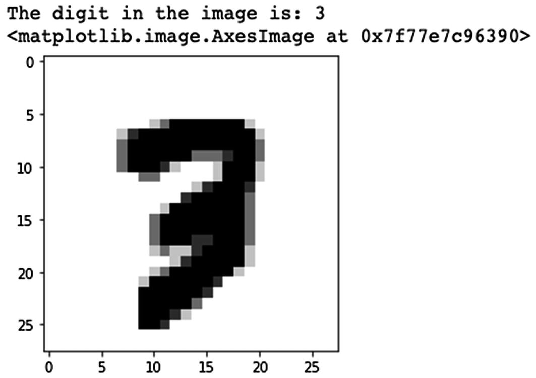
A Visualization of the Sample Image and Its Label

We also need to know the shape of the dataset to channel it to the convolutional neural network. Therefore, we use the shape attribute of the NumPy array with the following code:

x_train.shape

The output we get is (60000, 28, 28, 1). As you might have guessed, 60000 represents the number of images in the training dataset; (28, 28) represents the size of the image, 28 x 28 pixels; and 1 shows that our images are not colored.

Reshaping and Normalizing the Images

With TensorFlow’s dataset API, we already created a four-dimensional NumPy array for training, which is the required array dimension. On the other hand, we must normalize our data as it is a best practice in neural network models. We can achieve this by dividing the grayscale RGB codes to 255 (which is the maximum grayscale RGB code minus the minimum grayscale RGB code). This can be done with the following code:

# Making sure that the values are float so that we can get decimal points after division

x_train = x_train.astype('float32')

x_test = x_test.astype('float32')

# Normalizing the grayscale RGB codes by dividing it to the "max minus min grayscale RGB value".

x_train /= 255

x_test /= 255

print('x_train shape:', x_train.shape)

print('Number of images in x_train', x_train.shape[0])

print('Number of images in x_test', x_test.shape[0])

Building the Convolutional Neural Network

We build our model by using high-level Keras Sequential API to simplify the development process. I would like to mention that there are other high-level TensorFlow APIs such as Estimators, Keras Functional API, and another Keras Sequential API method, which helps us create neural networks with high-level knowledge. These different options may lead to confusion since they all vary in their implementation structure. Therefore, if you see entirely different codes for the same neural network, although they all use TensorFlow, this is why.

We use the most straightforward TensorFlow API – Keras Sequential API – since we don’t need much flexibility. Therefore, we import the Sequential model object from Keras and add Conv2D, MaxPooling, Flatten, Dropout, and Dense layers. We already covered Conv2D, MaxPooling, and Dense layers. In addition, Dropout layers fight with the overfitting by disregarding some of the neurons while training, while Flatten layers flatten two-dimensional arrays to a one-dimensional array before building the fully connected layers.

#Importing the required Keras modules containing model and layers

from tensorflow.keras.models import Sequential

from tensorflow.keras.layers import Dense,Conv2D, Dropout,Flatten,MaxPooling2D

#Creating a Sequential Model and adding the layers

model = Sequential()

model.add(Conv2D(28,kernel_size=(3,3), input_shape=(28,28,1)))

model.add(MaxPooling2D(pool_size=(2,2))

model.add(Flatten()) #Flattening the 2D arrays for fully connected layers

model.add(Dense(128,activation=tf.nn.relu))

model.add(Dropout(0.2))

model.add(Dense(10,activation=tf.nn.softmax))

We may experiment with any number for the first Dense layer; however, the final Dense layer must have 10 neurons since we have 10 number classes (0, 1, 2, …, 9). You may always experiment with kernel size, pool size, activation functions, dropout rate, and the number of neurons in the first Dense layer to get a better result.

Compiling and Fitting the Model

With the preceding code, we created a non-optimized empty CNN. Now it is time to set an optimizer with a given loss function which uses a metric. Then, we can fit the model by using our train data. We will use the following code for these tasks and see the outputs shown in Figure 7-7:

model.compile(optimizer='adam',

              loss='sparse_categorical_crossentropy',

              metrics=['accuracy'])

model.fit(x=x_train,y=y_train, epochs=10)

Output:

Figure 7-7

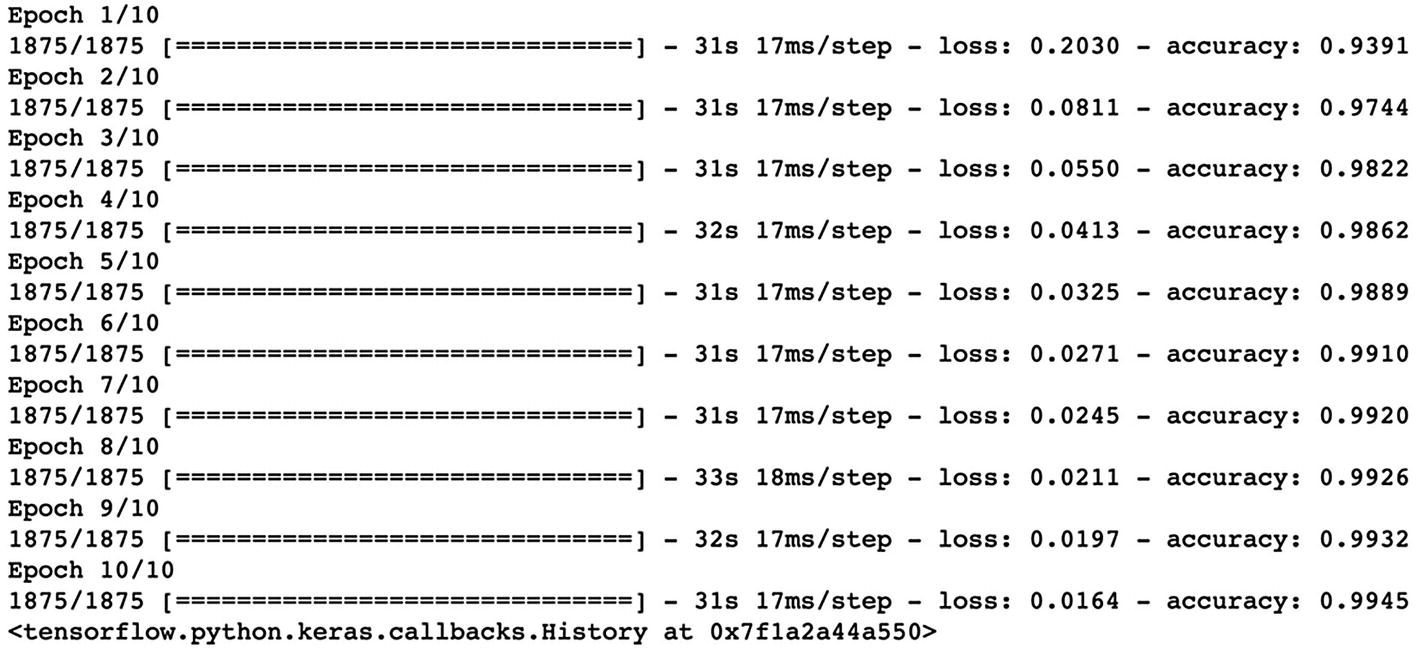
Epoch Stats for Our CNN Training on MNIST Dataset

You can experiment with the optimizer, loss function, metrics, and epochs. However, even though Adam optimizer, categorical crossentropy, and accuracy are the appropriate metrics, feel free to experiment.

Epoch number might seem a bit small. However, you can easily reach to 98–99% test accuracy. Since the MNIST dataset does not require substantial computing power, you may also experiment with the epoch number.

Evaluating the Model

Finally, you may evaluate the trained model with x_test and y_test using a single line of code:

model.evaluate(x_test, y_test)

The results in Figure 7-8 show the evaluation results for 10 epochs, calculated based on the test set performance.

Figure 7-8

Evaluation Results for Our MNIST-Trained CNN Model with 98.5% Accuracy

We achieved 98.5% accuracy with such a basic model. To be frank, in most image classification cases (e.g., for autonomous cars), we cannot even tolerate a 0.1% error. As an analogy, a 0.1% error can easily mean 1 accident in 1000 cases if we build an autonomous driving system. However, for our very first model, we can say that this result is outstanding.

We can also make individual predictions with the following code:

img_pred_index = 1000

plt.imshow(x_test[img_pred_index].reshape(28,28),

        cmap='Greys')

pred = model.predict(

                x_test[img_pred_index].reshape(1,28,28,1))

print("Our CNN model predicts that the digit in the image is:", pred.argmax())

Our trained CNN model will classify the image as the digit “5” (five), and here is the visual of the image in Figure 7-9.

Figure 7-9

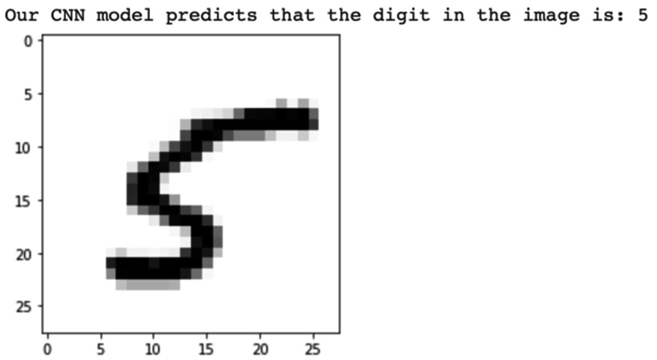
Our Model Correctly Classifies This Image as the Digit 5 (Five)

Please note that since we shuffle our dataset, you may see a different image for index 1000. But your model still predicts the digit with around 98% accuracy.

Although the image does not have good handwriting of the digit 5 (five), our model was able to classify it correctly.

Saving the Trained Model

In this case study, we built our first convolutional neural network to classify handwritten digits with Tensorflow’s Keras Sequential API. We achieved an accuracy level of over 98%, and now we can even save this model with the following lines of code:

# Save the entire model as a SavedModel.

# Create a 'saved_model' folder under the 'content' folder of your Google Colab Directory.

!mkdir -p saved_model

# Save the full model with its variables, weights, and biases.

model.save('saved_model/digit_classifier')

With the SavedModel, you can rebuild the trained CNN and use it to create different apps such as a digit-classifier game or an image-to-number converter!

Note

There are two types of saving options – the new and fancy “SavedModel” and the old “H5” format. If you would like to learn more about the differences between these formats, please take a look at the Save and Load section of the TensorFlow Guide:

www.tensorflow.org/tutorials/keras/save_and_load

Conclusion

Convolutional neural networks are very important and useful neural network models used mainly in image processing and classification. You can detect and classify objects in images, which may be used in many different fields such as anomaly detection in manufacturing, autonomous driving in transportation, and stock management in retail. CNNs are also useful to process audio and video as well as financial data. Therefore, the types of applications that take advantage of CNNs are even broader than the ones mentioned earlier.

CNNs consist of convolutional and pooling layers for feature learning and a set of fully connected layers for prediction and classification. CNNs reduce the complexity of the data, something that feedforward neural networks are not solely capable of.

In the next section, we will cover another essential neural network architecture: recurrent neural networks (RNNs), which are particularly useful for sequence data such as audio, video, text, and time-series data.