Once you have run the script from the preceding section, you should have 40,000 images for training in the cifar_10_images/data1/train directory and 8,000 images for validation in the cifar_10_images/data1/valid directory. We will train a model with this data. The code for this section is in the Chapter11/build_cifar10_model.R folder. The first section creates the model definition, which should be familiar to you:
library(keras)

# train a model from a set of images
# note: you need to run gen_cifar10_data.R first to create the images!
model <- keras_model_sequential()
model %>%
  layer_conv_2d(name="conv1", input_shape=c(32, 32, 3),
    filter=32, kernel_size=c(3,3), padding="same"
  ) %>%
  layer_activation("relu") %>%
  layer_conv_2d(name="conv2",filter=32, kernel_size=c(3,3),
                padding="same") %>%
  layer_activation("relu") %>%
  layer_max_pooling_2d(pool_size=c(2,2)) %>%
  layer_dropout(0.25,name="drop1") %>%

  layer_conv_2d(name="conv3",filter=64, kernel_size=c(3,3),
                padding="same") %>%
  layer_activation("relu") %>%
  layer_conv_2d(name="conv4",filter=64, kernel_size=c(3,3),
                padding="same") %>%
  layer_activation("relu") %>%
  layer_max_pooling_2d(pool_size=c(2,2)) %>%
  layer_dropout(0.25,name="drop2") %>%

  layer_flatten() %>%
  layer_dense(256) %>%
  layer_activation("relu") %>%
  layer_dropout(0.5) %>%
  layer_dense(256) %>%
  layer_activation("relu") %>%
  layer_dropout(0.5) %>%

  layer_dense(8) %>%
  layer_activation("softmax")

model %>% compile(
  loss="categorical_crossentropy",
  optimizer="adam",
  metrics="accuracy"
)
The model definition was adapted from the VGG16 architecture, which we will see later. I used a smaller number of blocks and fewer nodes. Note that the final dense layer must have 8 nodes, because there are only 8, not 10 classes in the data1 folder.
The next part sets up a data generator; the purpose of this is to load batches of image files into the model as it is being trained. We can also apply data augmentation to the train dataset in the data generator. We will select to create artificial data by randomly flipping the images horizontally, shifting images horizontally/vertically, and rotating the images by up to 15 degrees. We saw in Chapter 6, Tuning and Optimizing Models, that data augmentation can significantly improve existing models:
# set up data generators to stream images to the train function
data_dir <- "../data/cifar_10_images/"
train_dir <- paste(data_dir,"data1/train/",sep="")
valid_dir <- paste(data_dir,"data1/valid/",sep="")

# in CIFAR10
# there are 50000 images in training set
# and 10000 images in test set
# but we are only using 8/10 classes,
# so its 40000 train and 8000 validation
num_train <- 40000
num_valid <- 8000
flow_batch_size <- 50
# data augmentation
train_gen <- image_data_generator(
  rotation_range=15,
  width_shift_range=0.2,
  height_shift_range=0.2,
  horizontal_flip=TRUE,
  rescale=1.0/255)
# get images from directory
train_flow <- flow_images_from_directory(
  train_dir,
  train_gen,
  target_size=c(32,32),
  batch_size=flow_batch_size,
  class_mode="categorical"
)

# no augmentation on validation data
valid_gen <- image_data_generator(rescale=1.0/255)
valid_flow <- flow_images_from_directory(
  valid_dir,
  valid_gen,
  target_size=c(32,32),
  batch_size=flow_batch_size,
  class_mode="categorical"
)
Once the data generators have been set up, we will also use two callback functions. Callback functions allow you to run custom code after a specific number of batches / epochs have executed. You can write your own callbacks or use some predefined callback functions. Previously, we used callbacks for logging metrics, but here the callbacks will implement model checkpointing and early stopping, which are are often used when building complex deep learning models.
Model checkpointing is used to save the model weights to disk. You can then load the model from disk into memory and use it for predicting new data, or you can continue training the model from the point it was saved to disk. You can save the weights after every epoch, this might be useful if you are using cloud resources and are worried about the machine terminating suddenly. Here, we use it to keep the best model we have seen so far in training. After every epoch, it checks the validation loss, and if it is lower than the validation loss in the existing file, it saves the model.
Early stopping allows you to stop training a model when the performance no longer improves. Some people refer to it as a form of regularization because early stopping can prevent a model from overfitting. While it can avoid overfitting, it works very differently to the regularization techniques, such as L1, L2, weight decay, and dropout, that we saw in Chapter 3, Deep Learning Fundamentals. When using early stopping, you usually would allow the model to continue for a few epochs even if performance is no longer improving, the number of epochs allowed before stopping training is known as patience in Keras. Here we set it to 10, that is, if we have 10 epochs where the model has failed to improve, we stop training. Here is the code to create the callbacks that we will use in our model:
# call-backs
callbacks <- list(
  callback_early_stopping(monitor="val_acc",patience=10,mode="auto"),
  callback_model_checkpoint(filepath="cifar_model.h5",mode="auto",
                            monitor="val_loss",save_best_only=TRUE)
)
Here is the code to train the model:
# train the model using the data generators and call-backs defined above
history <- model %>% fit_generator(
  train_flow,
  steps_per_epoch=as.integer(num_train/flow_batch_size),
  epochs=100,
  callbacks=callbacks,
  validation_data=valid_flow,
  validation_steps=as.integer(num_valid/flow_batch_size)
)
One thing to note here is that we have to manage the steps per epoch for the train and validation generators. When you set up a generator, you don't know how much data is actually there, so we need to set the number of steps for each epoch. This is simply the number of records divided by the batch size.
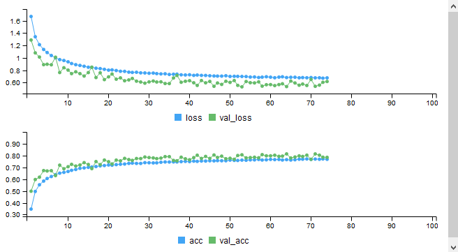
This model should take less than an hour to train on a GPU and significantly longer if training on a CPU. As the model is training, the best model is saved in cifar_model.h5. The best result on my machine was after epoch 64, when the validation accuracy was about 0.80. The model continued to train for another 10 epochs after this but failed to improve. Here is a plot of the training metrics: