Historically, one of the perceived disadvantages of using R for data science projects was the difficulty in deploying machine learning models built in R. This often meant that companies used R mainly as a prototyping tool to build models which were then rewritten in another language, such as Java and .NET. It is also one of the main reasons cited for companies switching to Python for data science as Python has more glue code, which allows it to interface with other programming languages.
Thankfully, this is changing. One interesting new product from RStudio, called RStudio Connect, allows companies to create a platform for sharing R-Shiny applications, reports in R Markdown, dashboards, and models. This allows companies to serve machine learning models using a REST interface.
The TensorFlow (and Keras) models we have created in this book can be deployed without any runtime dependency on either R or Python. One way of doing this is TensorFlow Serving, which is an open source software library for serving TensorFlow models. Another option is to use the Google CloudML interface that we saw in Chapter 10, Running Deep Learning Models in the Cloud. This allows you to create a publicly available REST API that can be called from your applications. TensorFlow models can also be deployed to iPhones and Android mobile phones.
There are two basic options for scoring models in production:
- Batch mode: In batch mode, a set of data is scored offline and the prediction results are stored and used elsewhere
- Real-time mode: In real-time mode, the data is scored immediately, usually a record at a time, and the results are immediately used.
For a lot of applications, batch mode is more than adequate. You should carefully consider if you really need a real-time prediction system as it is requires more resources and needs constant monitoring. It is much more efficient to score records in a batch rather than individually. Another advantage of batch mode is that you know the demand on the application beforehand and can plan resources accordingly. With real-time systems, a spike in demand or a denial of service attack can cause problems with your prediction model.
We have already seen batch mode for a saved model in the Using the saved deep learning model section in this chapter. So, let's look at how we can build a REST interface to get a prediction on new data from a deep learning model in real-time. This will use the tfdeploy package. The code for this section can be found in the Chapter11/deploy_model.R. We are going to build a simple model based on the MNIST dataset and then create a web interface where we can submit a new image for classification. Here is the first part of the code that builds the model and prints out the predictions for the first 5 rows in the test set:
library(keras)
#devtools::install_github("rstudio/tfdeploy")
library(tfdeploy)

# load data
c(c(x_train, y_train), c(x_test, y_test)) %<-% dataset_mnist()

# reshape and rescale
x_train <- array_reshape(x_train, dim=c(nrow(x_train), 784)) / 255
x_test <- array_reshape(x_test, dim=c(nrow(x_test), 784)) / 255

# one-hot encode response
y_train <- to_categorical(y_train, 10)
y_test <- to_categorical(y_test, 10)

# define and compile model
model <- keras_model_sequential()
model %>%
  layer_dense(units=256, activation='relu', input_shape=c(784),name="image") %>%
  layer_dense(units=128, activation='relu') %>%
  layer_dense(units=10, activation='softmax',name="prediction") %>%
  compile(
    loss='categorical_crossentropy',
    optimizer=optimizer_rmsprop(),
    metrics=c('accuracy')
  )

# train model
history <- model %>% fit(
  x_train, y_train,
  epochs=10, batch_size=128,
  validation_split=0.2
)
preds <- round(predict(model, x_test[1:5,]),0)
head(preds)
     [,1] [,2] [,3] [,4] [,5] [,6] [,7] [,8] [,9] [,10]
[1,]    0    0    0    0    0    0    0    1    0     0
[2,]    0    0    1    0    0    0    0    0    0     0
[3,]    0    1    0    0    0    0    0    0    0     0
[4,]    1    0    0    0    0    0    0    0    0     0
[5,]    0    0    0    0    1    0    0    0    0     0
There is nothing new about this code. Next, we will create a JSON file for one image file in the test set. JSON stands for JavaScript Object Notation, and is the accepted standard for serializing and sending data over a network connection. If HTML is the language for computers-to-human web communication, JSON is the language for computers-to-computers web communication. It is heavily used in microservice architecture, which is a framework for building a complex web ecosystem from lots of small web services. The data in the JSON file must have the same preprocessing applied as what was done during training – since we normalized the training data, we must also normalize the test data. The following code creates a JSON file with the values for the first instance in the testset and saves the file to json_image.json:
# create a json file for an image from the test set
json <- "{\"instances\": [{\"image_input\": ["
json <- paste(json,paste(x_test[1,],collapse=","),sep="")
json <- paste(json,"]}]}",sep="")
write.table(json,"json_image.json",row.names=FALSE,col.names=FALSE,quote=FALSE)
Now that we have a JSON file, let's create a REST web interface for our model:
export_savedmodel(model, "savedmodel")
serve_savedmodel('savedmodel', browse=TRUE)
Once you do this, a new web page should pop up that is similar to the following:
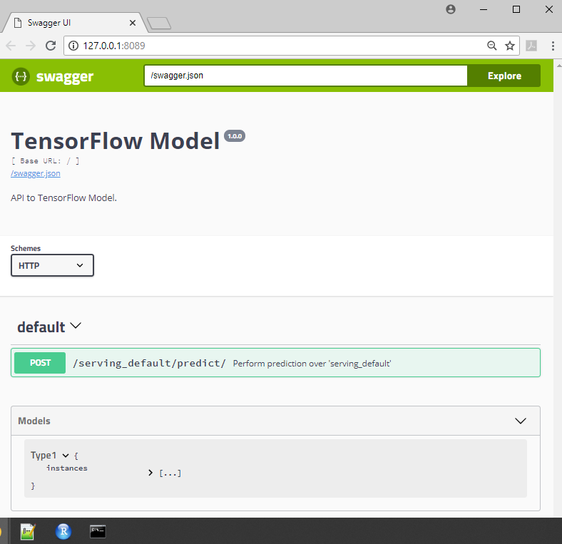
This is a Swagger UI page showing the RESTful web services for the TensorFlow model. This allows us to test our API. While we could try to use this interface, it is easier to use the JSON file we just created. Open up Command Prompt on your machine, browse to the Chapter11 code directory, and run the following command:
curl -X POST -H "Content-Type: application/json" -d @json_image.json http://localhost:8089/serving_default/predict
You should get the following response:

The REST web interface returns another JSON string with these results. We can see that the 8th entry in the list is 1.0 and that all the other numbers are extremely small. This matches the prediction for the first row that we saw in the code at the start of this section.