Now that we have built an auto-encoder and accessed the features of the inner layers, we will move on to an example of how auto-encoders can be used for anomaly detection. The premise here is quite simple: we take the reconstructed outputs from the decoder and see which instances have the most error, that is, which instances are the most difficult for the decoder to reconstruct. The code that is used here is in Chapter9/anomaly.R, and we will be using the UCI HAR dataset that we have already been introduced to in Chapter 2, Training a Prediction Model. If you have not already downloaded the data, go back to that chapter for instructions on how to do so.. The first part of the code loads the data, and we subset the features to only use the ones with mean, sd, and skewness in the feature names:
library(keras)
library(ggplot2)
train.x <- read.table("UCI HAR Dataset/train/X_train.txt")
train.y <- read.table("UCI HAR Dataset/train/y_train.txt")[[1]]
test.x <- read.table("UCI HAR Dataset/test/X_test.txt")
test.y <- read.table("UCI HAR Dataset/test/y_test.txt")[[1]]

use.labels <- read.table("UCI HAR Dataset/activity_labels.txt")
colnames(use.labels) <-c("y","label")

features <- read.table("UCI HAR Dataset/features.txt")
meanSD <- grep("mean\\(\\)|std\\(\\)|max\\(\\)|min\\(\\)|skewness\\(\\)", features[, 2])

train.x <- data.matrix(train.x[,meanSD])
test.x <- data.matrix(test.x[,meanSD])
input_dim <- ncol(train.x)
Now, we can build our auto-encoder model. This is going to be a stacked auto-encoder with two 40 neuron hidden encoder layers and two 40-neuron hidden decoder layers. For conciseness, we have removed some of the output:
# model
inner_layer_dim <- 40
input_layer <- layer_input(shape=c(input_dim))
encoder <- layer_dense(units=inner_layer_dim, activation='tanh')(input_layer)
encoder <- layer_dense(units=inner_layer_dim, activation='tanh')(encoder)
decoder <- layer_dense(units=inner_layer_dim)(encoder)
decoder <- layer_dense(units=inner_layer_dim)(decoder)
decoder <- layer_dense(units=input_dim)(decoder)

autoencoder <- keras_model(inputs=input_layer, outputs = decoder)
autoencoder %>% compile(optimizer='adam',
 loss='mean_squared_error',metrics='accuracy')
history <- autoencoder %>% fit(train.x,train.x,
 epochs=30, batch_size=128,validation_split=0.2)
Train on 5881 samples, validate on 1471 samples
Epoch 1/30
5881/5881 [==============================] - 1s 95us/step - loss: 0.2342 - acc: 0.1047 - val_loss: 0.0500 - val_acc: 0.1013
Epoch 2/30
5881/5881 [==============================] - 0s 53us/step - loss: 0.0447 - acc: 0.2151 - val_loss: 0.0324 - val_acc: 0.2536
Epoch 3/30
5881/5881 [==============================] - 0s 44us/step - loss: 0.0324 - acc: 0.2772 - val_loss: 0.0261 - val_acc: 0.3413
...
...

Epoch 27/30
5881/5881 [==============================] - 0s 45us/step - loss: 0.0098 - acc: 0.2935 - val_loss: 0.0094 - val_acc: 0.3379
Epoch 28/30
5881/5881 [==============================] - 0s 44us/step - loss: 0.0096 - acc: 0.2908 - val_loss: 0.0092 - val_acc: 0.3215
Epoch 29/30
5881/5881 [==============================] - 0s 44us/step - loss: 0.0094 - acc: 0.2984 - val_loss: 0.0090 - val_acc: 0.3209
Epoch 30/30
5881/5881 [==============================] - 0s 44us/step - loss: 0.0092 - acc: 0.2955 - val_loss: 0.0088 - val_acc: 0.3209
We can see the layers and number of parameters for the model by calling the summary function, like so:
summary(autoencoder)
_______________________________________________________________________
Layer (type)                 Output Shape                           Param #
=======================================================================
input_4 (InputLayer)         (None, 145)                            0
_______________________________________________________________________
dense_16 (Dense)             (None, 40)                             5840
_______________________________________________________________________
dense_17 (Dense)             (None, 40)                             1640
_______________________________________________________________________
dense_18 (Dense)             (None, 40)                             1640
_______________________________________________________________________
dense_19 (Dense)             (None, 40)                             1640
_______________________________________________________________________
dense_20 (Dense)             (None, 145)                            5945
=======================================================================
Total params: 16,705
Trainable params: 16,705
Non-trainable params: 0
_______________________________________________________________________
Our validation loss is 0.0088, which means that our model is good at encoding the data. Now, we will use the test set on the auto-encoder and get the reconstructed data. This will create a dataset with the same size as the test set. We will then select any instance where the sum of the squared error (se) between the predicted values and the test set is greater than 4.
These are the instances that the auto-encoder had the most trouble in reconstructing, and therefore they are potential anomalies. The limit value of 4 is a hyperparameter; if it is set higher, fewer potential anomalies are detected and if it is set lower, more potential anomalies are detected. This value would be different according to the dataset used.
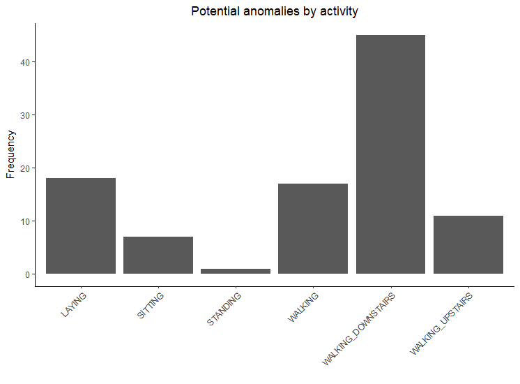
There are 6 classes in this dataset. We want to analyze if the anomalies are spread over all of our classes or if they are specific to some classes. We will print out a table of the frequencies of our classes in our test set, and we will see that the distribution of our classes is fairly even. When printing out a table of the frequencies of our classes of our potential anomalies, we can see that most of them are in the WALKING_DOWNSTAIRS class. The potential anomalies are shown in Figure 9.6:
# anomaly detection
preds <- autoencoder %>% predict(test.x)
preds <- as.data.frame(preds)
limit <- 4
preds$se_test <- apply((test.x - preds)^2, 1, sum)
preds$y_preds <- ifelse(preds$se_test>limit,1,0)
preds$y <- test.y
preds <- merge(preds,use.labels)
table(preds$label)
LAYING SITTING STANDING WALKING WALKING_DOWNSTAIRS WALKING_UPSTAIRS
   537     491      532     496                420              471

table(preds[preds$y_preds==1,]$label)
LAYING SITTING STANDING WALKING WALKING_DOWNSTAIRS WALKING_UPSTAIRS
    18       7        1      17                 45               11
We can plot this with the following code:
ggplot(as.data.frame(table(preds[preds$y_preds==1,]$label)),aes(Var1, Freq)) +
 ggtitle("Potential anomalies by activity") +
 geom_bar(stat = "identity") +
 xlab("") + ylab("Frequency") +
 theme_classic() +
 theme(plot.title = element_text(hjust = 0.5)) +
 theme(axis.text.x = element_text(angle = 45, hjust = 1, vjust = 1))
In this example, we used a deep auto-encoder model to learn the features of actimetry data from smartphones. Such work can be useful for excluding unknown or unusual activities, rather than incorrectly classifying them. For example, as part of an app that classifies what activity you engaged in for how many minutes, it may be better to simply leave out a few minutes where the model is uncertain or the hidden features do not adequately reconstruct the inputs, rather than to aberrantly call an activity walking or sitting when it was actually walking downstairs.
Such work can also help to identify where the model tends to have more issues. Perhaps further sensors and additional data are needed to represent walking downstairs or more could be done to understand why walking downstairs tends to produce relatively high error rates.
These deep auto-encoders are also useful in other contexts where identifying anomalies is important, such as with financial data or credit card usage patterns. Anomalous spending patterns may indicate fraud or that a credit card has been stolen. Rather than attempt to manually search through millions of credit card transactions, one could train an auto-encoder model and use it to identify anomalies for further investigation.