TensorFlow estimators allow you to build TensorFlow models using a simpler API interface. In R, the tfestimators package allows you to call this API. There are different model types, including linear models and neural networks. The following estimators are available:
- linear_regressor() for linear regression
- linear_classifier() for linear classification
- dnn_regressor() for deep neural network regression
- dnn_classifier() for deep neural network classification
- dnn_linear_combined_regressor() for deep neural network linear combined regression
- dnn_linear_combined_classifier() for deep neural network linear combined classification
Estimators hide a lot of the detail in creating a deep learning model, including building the graph, initializing variables and layers, and they can also integrate with TensorBoard. More details are available at https://tensorflow.rstudio.com/tfestimators/. We will use dnn_classifier with the data from the binary classification task from Chapter 4, Training Deep Prediction Models. The following code in the Chapter8/tf_estimators.R folder demonstrates TensorFlow estimators.
- We only include the code that is specific to TensorFlow estimators and omit the code at the start of the file that loads the data and splits it into train and test data:
response <- function() "Y_categ"
features <- function() predictorCols

FLAGS <- flags(
  flag_numeric("layer1", 256),
  flag_numeric("layer2", 128),
  flag_numeric("layer3", 64),
  flag_numeric("layer4", 32),
  flag_numeric("dropout", 0.2)
)
num_hidden <- c(FLAGS$layer1,FLAGS$layer2,FLAGS$layer3,FLAGS$layer4)

classifier <- dnn_classifier(
  feature_columns = feature_columns(column_numeric(predictorCols)),
  hidden_units = num_hidden,
  activation_fn = "relu",
  dropout = FLAGS$dropout,
  n_classes = 2
)

bin_input_fn <- function(data)
{
 input_fn(data, features = features(), response = response())
}
tr <- train(classifier, input_fn = bin_input_fn(trainData))
[\] Training -- loss: 22.96, step: 2742

tr
Trained for 2,740 steps.
Final step (plot to see history):
 mean_losses: 61.91
total_losses: 61.91
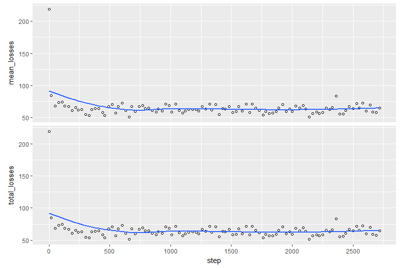
- Once the model is trained, the following code plots the training and validation metrics:
plot(tr)
- This produces the following plot:
- The next part of the code calls the evaluate function to produce metrics for the model:
# predictions <- predict(classifier, input_fn = bin_input_fn(testData))
evaluation <- evaluate(classifier, input_fn = bin_input_fn(testData))
[-] Evaluating -- loss: 37.77, step: 305

for (c in 1:ncol(evaluation))
 print(paste(colnames(evaluation)[c]," = ",evaluation[c],sep=""))
[1] "accuracy = 0.77573162317276"
[1] "accuracy_baseline = 0.603221416473389"
[1] "auc = 0.842994153499603"
[1] "auc_precision_recall = 0.887594640254974"
[1] "average_loss = 0.501933991909027"
[1] "label/mean = 0.603221416473389"
[1] "loss = 64.1636199951172"
[1] "precision = 0.803375601768494"
[1] "prediction/mean = 0.562777876853943"
[1] "recall = 0.831795573234558"
[1] "global_step = 2742"
We can see that we got an accuracy of 77.57%, which is actually almost identical to the accuracy we got on the MXNet model in Chapter 4, Training Deep Prediction Models, which had a similar architecture. The dnn_classifier() function hides a lot of the detail, so Tensorflow estimators are a good way to use the power of TensorFlow for tasks with structured data.
Models created using TensorFlow estimators can be saved onto disk and loaded later. The model_dir() function shows the location of where the model artifacts were saved (usually in a temp directory, but it can be copied elsewhere):
model_dir(classifier)
"C:\\Users\\xxxxxx\\AppData\\Local\\Temp\\tmpv1e_ri23"
# dnn_classifier has a model_dir parameter to load an existing model
?dnn_classifier
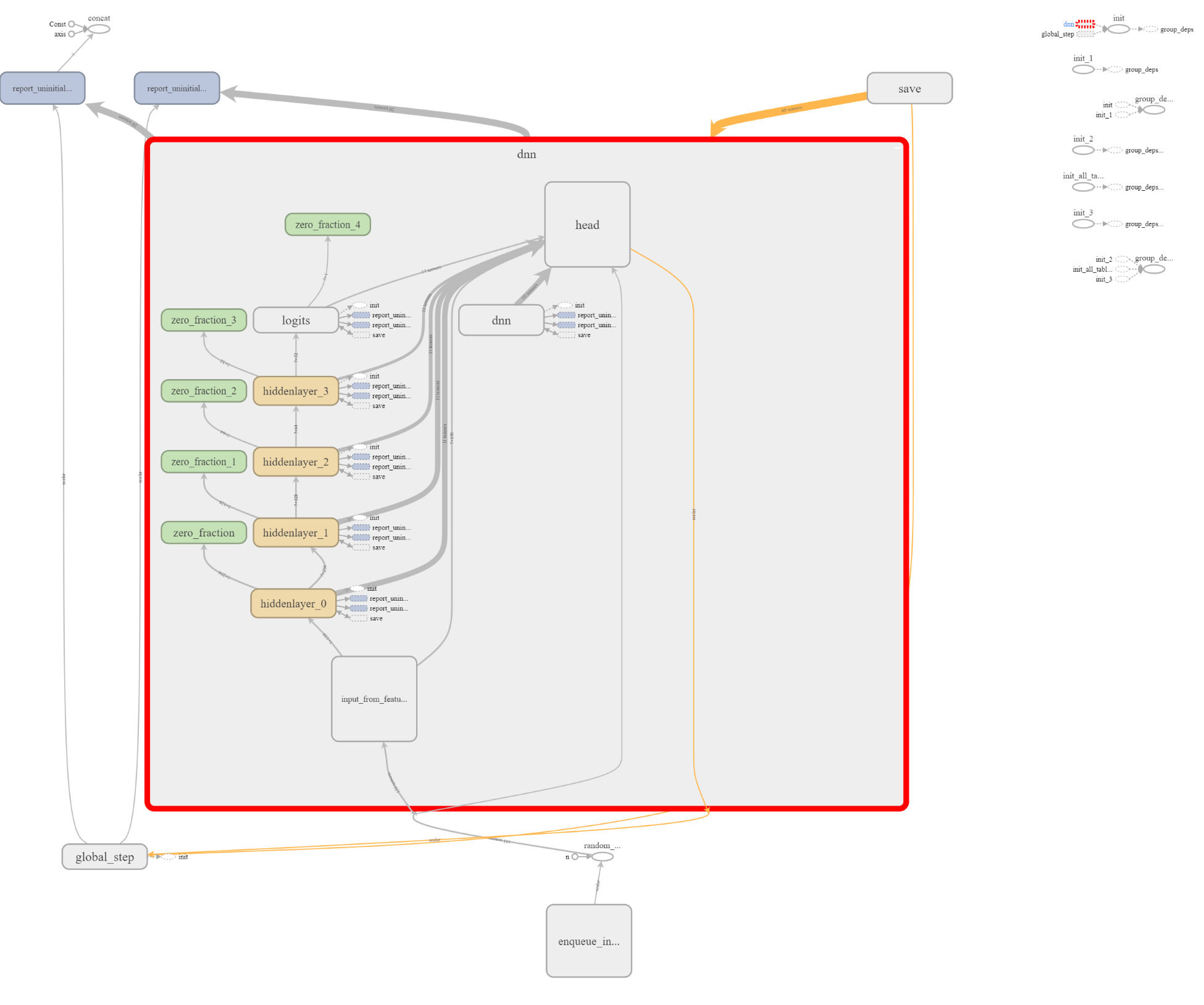
Included in the model artifacts are the event logs that can be used by TensorBoard. For example, when I load TensorBoard up and point it to the logs directory in the temp directory, I can see the TensorFlow graph that was created: