9
Impact of Quantum Computing

It is, of course, impossible to predict the long-term impact of quantum computing with any accuracy. If we look back at the birth of the modern computer in the 1950s, nobody could have predicted how much computers would change society and how dependent we would become on them. There are well-known quotes from computer pioneers proclaiming that the world would only need a handful of computers and that nobody would ever need a computer in their home. These quotes are out of context. The authors were generally referring to specific types of computers, but the impression they give, though exaggerated, is true. Initially computers were massive, had to be in air-conditioned rooms, and were not very reliable. Today, I have a laptop, a smartphone, and a tablet. All three are far more powerful than the first computers. I think that even visionaries like Alan Turing would be amazed at the extent to which computers have thoroughly permeated all levels of society. Turing did discuss chess playing and artificial intelligence, but nobody predicted that the rise of e-commerce and social media would come to dominate so much of our lives.

Quantum computing is now in its infancy, and the comparison to the first computers seems apt. The machines that have been constructed so far tend to be large and not very powerful, and they often involve superconductors that need to be cooled to extremely low temperatures. Already there are some people saying that there will be no need for many quantum computers to be built and that their impact on society will be minimal. But, in my opinion, these views are extremely shortsighted. Although it is impossible to predict what the world will be like in fifty years time, we can look at the dramatic changes in quantum computing over the last few years and see the direction in which it is heading. It might be some time before we get powerful universal quantum computers, but even before we do, quantum computing looks likely to make a substantial impact on our lives. In this chapter we will look at some ways that this could occur. In contrast to the previous chapter where we looked at three algorithms in considerable depth, we will look at a wide variety of topics at a less detailed level.

Shor’s Algorithm and Cryptanalysis

The major result in quantum computing concerning cryptanalysis is Shor’s algorithm. To fully understand this algorithm requires a substantial mathematics background. It uses Euler’s theorem and continued fraction expansions from number theory. It also requires knowledge of complex analysis and the discrete Fourier transform. It marks the place where the theory of quantum computation changes from requiring just elementary mathematics to a more substantial background. Consequently, we won’t be covering the algorithm in detail, but its importance means that we should at least look at it.

It is an algorithm, like Simon’s algorithm, that has a quantum part and a classical part. The quantum part is similar to that of Simon’s algorithm. Before we give a brief description, we will look at the problem that Shor wanted to tackle.

RSA Encryption

The RSA encryption method is named after its inventors, Ron Rivest, Adi Shamir, and Leonard Adleman. They published a paper on it and then patented it in 1978. Later it became known that Clifford Cocks, working for the Government Communications Headquarters (GCHQ), a British intelligence agency, had essentially invented the same algorithm in 1973. The British classified it, but they did pass it on to the Americans. It seems, however, that neither of the American or British intelligence agencies used it or realized how important it would become. Nowadays, it is used widely on the Internet for encrypting data sent from one computer to another. It is used for Internet banking and for electronic purchases using credit cards.

We will show how the encryption algorithm works with an example in which we want to share some confidential information with our bank and, at the same time, want to protect it from anyone who might be eavesdropping.

When you want to communicate with the bank, you want to encrypt your data so that if it is intercepted it cannot be read. The actual encryption of the data is going to be done using a key that both you and the bank share to both encrypt and decrypt—this is called a symmetric key—and must be kept secret by both parties. The key is generated on your computer and sent to the bank, but, of course, we can’t just send the key without encrypting it. We need to encrypt the key that we are going to use to encrypt our communication with the bank. This is where RSA encryption enters the picture. It is a way of securely sending the key to the bank.

To start the communication with the bank, your computer generates the key that will be used later for encryption and decryption for both you and the bank. We will call the key K.

The bank’s computer finds two large prime numbers that we will denote by p and q. The primes need to be roughly the same size and the product N = pq, called the modulus, should contain at least 300 digits using standard decimal numbers (1024 binary digits), which is currently considered large enough to ensure security. This is fairly straightforward. There are efficient ways of generating these primes and multiplying the two primes to get the modulus N is easy.

The second step is for the bank to find a relatively small number e that shares no common factors with either or . This is also easy to compute. The bank keeps the primes p and q secret, but sends the numbers N and e.

Your computer takes the key K and raises it to the power e taking the remainder after dividing by N. Once more, this is easy to do. This is the number is called mod N. This is then sent to the bank. The bank knows how to factor N into p and q, and this lets it quickly calculate K.

If someone is tapping into the communication, they will know N and e, both of which the bank sent, they will also know the number mod N that you sent. To calculate K, the eavesdropper needs to know the factors p and q of N, but these are being kept secret. The security of the system depends on the fact that the eavesdropper will not be able to factor the number N to obtain p and q.

The question is how hard is it to factor a number that is the product of two large primes? The answer is that it seems hard. All of the other steps involved in RSA encryption can be performed with classical algorithms that take polynomial time, but nobody has discovered a classical algorithm that can factor a product of two large primes in polynomial time. But, on the other hand, nobody has a proof that such an algorithm doesn’t exist.

This is where Shor enters the picture. He constructed a quantum algorithm that does factor a product of large prime numbers. The algorithm belongs to class BQP, which means that it works with bounded error in polynomial time. One thing that needs to be emphasized is that we are no longer talking about query complexity. We are not assuming that we can ask questions of an oracle. We are counting the total number of steps or, equivalently, the time needed to get from the beginning to the end of the computation. Shor is giving a concrete algorithm for each step. The fact that the algorithm belongs to BQP means that if it is implemented it becomes feasible to factor large numbers, and, more important, it means that if the quantum circuit can be actually constructed, then RSA encryption is no longer secure.

Shor’s Algorithm

Shor’s algorithm involves a significant amount of mathematics. We will just give a short and somewhat vague description of the quantum part.

An important part of the algorithm is a gate that is called the quantum Fourier transform gate. This can be thought of as a generalization of the Hadamard gate. In fact, for one qubit the quantum Fourier transform gate is exactly H. Recall that we used a recursive formula that told us how to get from the matrix for to the matrix for . Similarly, we can give a recursive formula for the quantum Fourier transform matrix. The major difference between and the quantum Fourier matrix is that the entries in the latter case are generally complex numbers—more specifically, they are complex roots of unity. Recall that the entries for are either 1 or . These are the two possible square roots of 1. When we look for fourth roots of 1 we again just get if we are using real numbers, but we get two other roots if we use the complex numbers. In general, 1 has n complex nth roots. The quantum Fourier transform matrix on n qubits involves all the th complex roots of unity.

Simon’s algorithm was based on the properties of . It used interference, the amplitudes were either 1 or which meant that when we added terms, the kets either canceled or reinforced one another. Shor realized that a similar idea applied to the quantum Fourier matrix, only now the amplitudes are given not just by 1 and , but also by all the th complex roots of unity, which means that we can detect more types of periods than just the ones that Simon’s algorithm considers.

Recall that we know the number N and want to factor it into the product of the two primes p and q. The algorithm chooses a number a satisfying . It checks to see if a shares any factors with N, if it does we can deduce that a is a multiple of either p or q. From there it is easy to complete the factorization. If a does not share any factors with N, then we calculate a mod(N), mod(N), mod(N), and so on, where mod(N) means calculate and then take the remainder when divided by N. Since these numbers are remainders, they will all be less than N. Consequently, this sequence of numbers will eventually repeat. There will be some number r such that . The number r can be thought of as the period, and it is this number that the quantum part of Shor’s algorithm computes. Once r has been found, classical algorithms can use this fact to determine the factors of N.

Well, that description was rather sketchy, but it gives some idea of how the quantum part of Shor’s algorithm works. The key part is that Simon’s algorithm for finding the secret string s can be generalized to find the unknown period r.

The algorithm actually has been implemented, but just for small numbers. In 2001, it was used to factor 15 and in 2012 it factored 21. Clearly, it is nowhere near factoring 300 digit numbers at the moment. But how long will it take before a circuit can be built for numbers of this size? It seems to be only a matter of time until the RSA encryption scheme will no longer be secure.

Over the years other methods of encryption have been developed, but Shor’s algorithm also works on many of these. It has become clear that we need to develop new cryptographic methods—and these new methods should be able to withstand not just classical attacks but also attacks by quantum computers.

Post-quantum cryptography is now an extremely active area, with new methods of encryption being developed. Of course, there is no reason why these have to use quantum computing. We just need the encrypted message to be able to withstand being broken by a quantum computer. But quantum ideas do give us ways of constructing secure codes.

We have seen two quantum key distribution (QKD) schemes that are secure: the BB84 and Ekert’s protocols. Several labs have succeeded in getting QKD systems up and running. There are also a few companies that offer QKD systems for sale. One of the first times that QKD was used in a real-world setting was in 2007, when ID Quantique set up a system to secure the transmission of votes between a counting station and Geneva’s main polling office during a Swiss parliamentary election.

Many countries are experimenting with small quantum networks using optic fiber. There is the potential of connecting these via satellite and being able to form a worldwide quantum network. This work is of great interest to financial institutions.

The most impressive results, so far, involve a Chinese satellite that is devoted to quantum experiments. It’s named Micius after a Chinese philosopher who did work in optics. This is the satellite that was used for the quantum teleportation we mentioned in an earlier chapter. It has also been used for QKD. A team in China connected to a team in Austria—the first time that intercontinental QKD has been achieved. Once the connection was secured, the teams sent pictures to one another. The Chinese team sent the Austrians a picture of Micius, and the Austrians sent a picture of Schrödinger to the Chinese.

Grover’s Algorithm and Searching Data

We are entering the era of big data. Searching through enormous data sets efficiently is now a high priority for many major companies. Grover’s algorithm has the potential to speed up data searches.

Lov Grover invented the algorithm in 1996. Like Deutsch’s and Simon’s algorithms, its speedup over classical algorithms is given in terms of query complexity. Of course, to implement the algorithm for real-world data searches, we don’t have oracles that can answer our questions. We have to construct an algorithm that does the work of the oracle. But before we begin to discuss how to implement Grover’s algorithm, we will look at what it does and how it does it.

Grover’s Algorithm

Imagine that you have four cards in front of you. They are all face down. You know that one of them is the ace of hearts, and this is the card you want to find. How many cards must you turn over until you know the location of the ace of hearts?

You might be lucky and turn it over on the first try, or you might be unlucky and turn over three cards, none of which is the ace. If you are unlucky and haven’t turned it over after three tries, then you know that the last card must be the ace. So, we know where the ace is after turning over between one and three cards. On average we have to turn over 2.25 cards.

This problem is one that Grover’s algorithm tackles. Before we begin describing the algorithm, we will reword the problem. We have four binary strings: 00, 01, 10, and 11. We have a function f that sends three of these strings to 0 and the other one to 1. We want to find the find the binary string that is sent to 1. For example, we might have , , , and . The problem now asks how many function evaluations do we need to make before we find that . We are just restating the problem, wording it in terms of functions instead of cards, so we know the answer is the same as before: 2.25 on average.

As with all query complexity algorithms we construct an oracle—a gate that encapsulates the function. For our example, where we just have four binary strings, the oracle is given in figure 9.1.

The circuit for Grover’s algorithm is given in figure 9.2.

The algorithm has two steps. The first is to flip the sign of the probability amplitude connected to the location we are trying to find. The second is to amplify this probability amplitude. We will show how the circuit does this.

After going through the Hadamard gates, the top two qubits will be in state

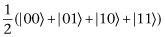
and the bottom qubit will be in state

We can write the combined state as

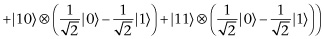The qubits then pass through the F gate. This flips and of the third qubit in the location we are trying to find. If we use our example where , we obtain

This can be written as

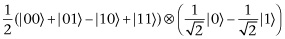The result is that the top two qubits are not entangled with the bottom qubit, but we have flipped the sign of the probability amplitude of , which corresponds to the location we are trying to find.

At this stage, if we were to measure the top two qubits we would get one of the four locations, with each of the four answers being equally likely. We need another trick and that is amplitude amplification. Amplitude amplification works by flipping a sequence of numbers about their mean. If a number is above the mean, it is flipped below the mean. If a number is below the mean, it is flipped above the mean. In each case the distance to the mean is preserved. To illustrate, we use the four numbers 1, 1, 1, and . Their sum is 2, and so their mean is 2/4, which is equal to 1/2. We then go through the sequence of numbers. The first is 1. This is 1/2 above the mean. When we flip about the mean it becomes 1/2 below the mean. In this case it becomes 0. The number is 3/2 below the mean. When we flip about the mean it becomes 3/2 above the mean, which is 2.

Our top two qubits are currently in the state

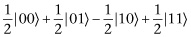If we flip the probability amplitudes about the mean we get 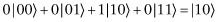. When we measure this we will get 10 with certainty, so flipping about the mean does exactly what we want. We just need to make sure that there is a gate or, equivalently, an orthogonal matrix that performs the flip about the mean. There is. It’s

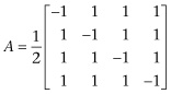When this gate acts on the top two qubits we get

For this example, where we just have two qubits, we only need to use the oracle once. We only need to ask one question. So, for , Grover’s algorithm gives the answer with certainty with just one question, whereas the classical case takes 2.25 questions on average.

Exactly the same idea works for n qubits. We start by flipping the sign of the probability amplitude that corresponds to the location we are trying to find. Then we flip about the mean. However, the amplitude magnification is not as dramatic in general as in the case for just two qubits. For example, if we have eight numbers, seven of which are 1 and the other of which is . Their sum is 6, and so their mean is 6/8. When we flip about the mean, the 1s become 1/2s, and the becomes 10/4. The consequence of this is that if we have three qubits, after performing the amplitude magnification, if we were to measure our qubits, we would get the location we are trying to find with higher probability than the other locations. The concern is that there is still some significant probability that we will get the wrong answer. We want a higher probability of getting the right answer—we want to magnify the amplitude even more before we measure. The solution is that we send everything back through the circuit. We flip the sign of the probability amplitude associated with the location we are trying to find again and then perform the flip about the mean again.

Let’s look at the general case. We want to find something that could be in one of m possible locations. To find it classically we need to ask questions in the worst-case scenario. The number of questions grows at the same rate as the size of m. Grover calculated a formula for the number of times you should use his circuit to maximize the chance of getting the correct answer. The number given by this formula grows at the rate . This is a quadratic speedup.

Applications of Grover’s Algorithm

There are a number of problems with implementing the algorithm. The first is that the quadratic speedup is for query complexity. If we need to use an oracle, then we need to actually construct it, and if we are not careful the number of steps involved with the computation of the oracle will outweigh the number of steps saved by the algorithm, resulting in the algorithm being slower rather than faster than the classical one. Another problem is that in calculating the speedup we are assuming that there is no underlying order to the data set. If there is structure, we can often find classical algorithms that exploit the structure and find the solution more quickly than randomly guessing. The last concern is about the speedup. Quadratic speedup is nothing like the exponential speedup we have seen with other algorithms. Can’t we do better? Let’s look at these concerns.

The concerns involving implementing the oracle and the structure of data sets are both valid and show that Grover’s algorithm is not going to be practical for most database searches. But in certain cases the structure of the data can make it possible to construct an oracle that works efficiently. In these cases, the algorithm can give a speedup over classical algorithms. The question about whether we can do better than quadratic speedup has been answered. It has been proved that Grover’s algorithm is optimal. There is no quantum algorithm that can solve the problem with more than just quadratic speedup. Quadratic speedup, though not as impressive as exponential speedup, is useful. With massive data sets, any speedup can be valuable.

The main applications for Grover’s algorithm are probably not going to be for the algorithm as has been presented but for variations on it. In particular, the idea of amplitude amplification is a useful one.

We have only presented a few algorithms, but Shor’s and Grover’s are considered the most important. Many other algorithms have built upon the ideas in these two.* We now turn our attention from algorithms to other applications of quantum computing.

Chemistry and Simulation

In 1929, Paul Dirac wrote about quantum mechanics, saying, “The fundamental laws necessary for the mathematical treatment of a large part of physics and the whole of chemistry are thus completely known, and the difficulty lies only in the fact that the application of these laws leads to equations that are too complex to be solved.”

In theory, all of chemistry involves interactions of atoms and configurations of electrons. We know the underlying mathematics—it’s quantum mechanics, but although we can write down the equations we cannot solve them exactly. In practice, chemists use approximation techniques instead of trying to find exact solutions. These approximations ignore fine details. Computational chemistry has taken this approach and, in general, it has worked well. Classical computers can give us good answers in many cases, but there are areas where the current computational techniques don’t work. The approximation is not good enough. You need the fine details.

Feynman thought that one of the main applications of quantum computers would be to simulate quantum systems. Using quantum computers to study chemistry that belongs to the quantum world is a natural idea that has great potential. There are a number of areas where it is hoped that quantum computing will make important contributions. One of these is to understand how an enzyme, nitrogenase, used to make fertilizers actually works. The current method of producing fertilizers releases a significant amount of greenhouse gases and consumes considerable energy. Quantum computers could play a major role in understanding this and other catalytic reactions.

There is a group at the University of Chicago that is looking into photosynthesis. The transfer of sunlight to chemical energy is a process that happens quickly and very efficiently. It is a quantum mechanical process. The long-term goal is to understand this process and then use it in photovoltaic cells.

Superconductivity and magnetism are quantum mechanical phenomena. Quantum computers may help us understand them better. One goal is to develop superconductors that don’t need to be cooled to near absolute zero.

The actual construction of quantum computers is in its infancy, but even with a few qubits it is possible to begin studying chemistry. IBM recently simulated the molecule beryllium hydride (BeH₂) on a seven-qubit quantum processor. This is a relatively small molecule with just three atoms. The simulation does not use the approximations that are used in the classical computational approach. However, since IBM’s processor uses just a few qubits, it is possible to simulate the quantum processor using a classical computer. Consequently, everything that can be done on this quantum processor can be done classically. However, as processors incorporate more qubits we get to the point where it is no longer possible to simulate them classically. We will soon be entering a new era when quantum simulations are beyond the power of any classical computer.

Now that we have seen some of the possible applications, we will briefly survey some of the ways that are being used to build quantum computers.

Hardware

To actually make practical quantum computers you need to solve a number of problems, the most serious being decoherence—the problem of your qubit interacting with something from the environment that is not part of the computation. You need to set a qubit to an initial state and keep it in that state until you need to use it. You also need to be able to construct gates and circuits. What makes a good qubit?

Photons have the useful properties of being easy to initialize and easy to entangle, and they don’t interact very much with the environment, so they stay coherent for long times. On the other hand, it is difficult to store photons and have them ready when you need them. The properties of photons make them ideal for communication, but they are more problematic for building quantum circuits.

We have often used electron spin as an example. Can this be used? Earlier we mentioned the apparatus used in the loophole-free Bell test. It used electrons trapped in synthetic diamonds. These are manipulated by shining lasers on them. The problem has been scaling. You can construct one or two qubits but, at the moment, it is not possible to generate large numbers. Instead of using electrons, spins of the nucleus have also been tried, but scalability is again the problem.

Another method uses the energy levels of ions. Ion-trap computing uses ions that are held in position by electromagnetic fields. To keep the ions trapped vibrations must be minimized; cooling everything to near absolute zero does this. The ions’ energy levels encode the qubits and lasers can manipulate these. David Wineland used ion traps to construct the first CNOT gate in 1995, for which he received a Nobel Prize, and in 2016 researchers at NIST entangled more than 200 beryllium ions. Ion-traps do have potential to be used in future quantum computers, but a number of computers are being constructed using a different approach.

To minimize the interaction of quantum computers with the environment, they are always protected from light and heat. They are shielded against electromagnetic radiation, and they are cooled. One thing that can happen in cold places is that certain materials become superconductors—they lose all electrical resistance—and superconductors have quantum properties that can be exploited. These involve things called Cooper pairs and Josephson junctions.

The electrons in a superconductor pair up, forming what are called Cooper pairs. These pairs of electrons act like individual particles. If you sandwich thin layers of a superconductor between thin layers of an insulator, you obtain a Josephson junction.** These junctions are now used in physics and engineering to create sensitive instruments for measuring magnetic fields. For our purposes, the important fact is that the energy levels of the Cooper pairs in a superconducting loop that contains a Josephson junction are discrete and can be used to encode qubits.

IBM uses superconducting qubits in its quantum computers. In 2016, IBM introduced a five-qubit processor that they have made available to everyone for free on the cloud. Anyone can design their own quantum circuit, as long as it uses five or fewer qubits, and run it on this computer. IBM’s aim is to introduce quantum computing to a wide audience—circuits for superdense coding, for Bell’s inequality, and a model of the hydrogen atom have all been run on this machine. A primitive version of Battleships has also been run, giving the coder the claim of constructing the first quantum computer multiplayer game. At the end of 2017, IBM connected a twenty-qubit computer to the cloud. This time it is not for education, but it is a commercial venture where companies can buy access.

Google is working on its quantum computer. It also uses superconducting qubits. Google is expected to announce in the near future that it has a computer that uses 72 qubits. What is special about this number?

Classical computers can simulate quantum computers if the quantum computer doesn’t have too many qubits, but as the number of qubits increases we reach the point where that is no longer possible. Google is expected to announce that it has reached or exceeded this number, giving them the right to claim quantum supremacy—the first time an algorithm has been run on a quantum computer that is impossible to run, or simulate, on a classical computer. IBM, however, is not giving up without a fight. Its team, using some innovative ideas, has recently found a way to simulate a 56-qubit system classically, increasing the lower bound on the number of qubits needed for quantum supremacy.

As work continues on building quantum computers, we are likely to see spinoffs into other areas. Qubits, however we encode them, are sensitive to interactions with their surroundings. As we understand these interactions better we will be able to build better shields to protect our qubits, but we will also be able to design ways our qubits can measure their surroundings. An example involves electrons trapped in synthetic diamonds. These are very sensitive to magnetic fields. NVision Imaging Technologies is a startup that is using this idea to build NMR machines that they hope will be better, faster, and cheaper than current ones.

Quantum Annealing

D-Wave has computers for sale. Their latest, the D-Wave 2000Q has, as you might guess from its name, 2,000 qubits. However, their computers are not general purpose, they are designed for solving certain optimization problems using quantum annealing. We will give a brief description of this.

Blacksmiths often need to hammer metal and bend metal. In the process, it can become hardened—various stresses and deformities occur in the crystal structure—making it hard to work. Traditional annealing is a method of restoring the uniform crystal structure, making the metal malleable once more. It’s done by heating the piece of metal to a high temperature and then letting it slowly cool.

Simulated annealing is a standard technique, based on annealing, that can be used for solving certain optimization problems. For example, suppose we have the graph given in figure 9.3 and want to find the lowest point—the absolute minimum. Think of the graph as being the bottom of a two-dimensional bucket. We drop a ball bearing into the bucket. It will settle at the bottom of one of the valleys. These are labeled A, B, and C in the figure. We want to find C. The ball bearing may not land at the bottom of C, but instead it might end up at the bottom of valley at A. The important observation in annealing is that the energy required to push the ball bearing up the hill and let it drop into valley B is much less than the energy needed to push the ball bearing up from B and let it drop into A. So, we shake the bucket with an energy level between these two values. The ball can move from A to B, but it cannot move back. After a while of shaking at this level, it will end up either at the bottom of A or B. But shaking at this level can send the ball from C to B. The next step is to shake it again, but less energetically, with enough energy to get it up the peak from B to C, but not enough to let it get back from C to B.

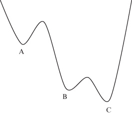
Figure 9.3 Graph of function—bottom of bucket.

In practice, you start shaking and gradually reduce the energy. This corresponds to gradually cooling your piece of metal in traditional annealing. The result is that the ball bearing ends up at the lowest point. You have found the absolute minimum of the function.

Quantum annealing adds quantum tunneling. This is a quantum effect where the ball bearing can just appear on the other side of a hill. Instead of going over, it can go through. Instead of reducing the heights of hills the ball can climb, you reduce the length of the tunnels it can tunnel through.

D-Wave has produced a number of commercially available computers that use quantum annealing for optimization problems. Initially, they were met with some skepticism about whether the computers actually used quantum tunneling, but now it is generally agreed that they do. There is still some question of whether the computers are faster than classical ones, but people are buying. Volkswagen, Google, and Lockheed Martin, among others, have all bought D-Wave machines.

After this brief look at hardware, we turn to deeper questions. What does quantum computation tell us about us, the universe, and what computation is at its most fundamental level?

Quantum Supremacy and Parallel Universes

There are 8 possible three-bit combinations: 000, 001, 010, 011, 100, 101, 110, 111. The number 8 comes from . There are two choices for the first bit, two for the second and two for the third, and we multiply these three 2s together. If instead of bits we switch to qubits, each of these 8 three-bit strings is associated with a basis vector, so the vector space is 8-dimensional. Exactly the same analysis tells us that if we have n qubits, then we will have basis vectors, and the space will be -dimensional. As the number of qubits grows, the number of basis vectors grows exponentially, and things quickly get big.

If we have 72 qubits, the number of basis elements is . This is about 4,000,000,000,000,000,000,000. It is a large number and is considered to be around the point at which classical computers cannot simulate quantum computers. Once quantum computers have more than 72 or so qubits we will enter the age of quantum supremacy—when quantum computers can do computations that are beyond the ability of any classical computer. As we mentioned earlier, it is expected that Google is about to announce that this age has been reached. (D-Wave has 2,000 qubits in its latest computer. However, this specialized machine has not been able to do anything that cannot be done by a conventional computer, so it hasn’t broken the quantum supremacy barrier.)

Let’s consider a machine with 300 qubits. This doesn’t seem an unreasonable number for the not too distant future. But is an enormous number. It’s more than the number of elementary particles in the known universe! A computation using 300 qubits would be working with basis elements. David Deutsch asks where computations like this, which involve more basis elements than there are particles in the universe, are done. He believes that we need to introduce parallel universes, each collaborating with one another.

This view of quantum mechanics and parallel universes goes back to Hugh Everett. Everett’s idea is that, whenever we make a measurement, the universe splits into several copies, each containing a different outcome. Though this is distinctly a minority view, Deutsch is a firm believer. His paper in 1985 is one of the foundational papers in quantum computing, and one of Deutsch’s goals with this work was to make a case for parallel universes. He hopes that one day that there will be a test, analogous to Bell’s test, that will confirm this interpretation.

Computation

Alan Turing is one of the fathers of the theory of computation. In his landmark paper of 1936 he carefully thought about computation. He considered what humans did as they performed computations and broke it down to its most elemental level. He showed that a simple theoretical machine, which we now call a Turing machine, could carry out any algorithm. Turing’s theoretical machines evolved into our modern day computers. They are universal computers. Turing’s analysis showed us the most elemental operations. These involve the manipulation of bits. But remember, Turing was analyzing computation based on what humans do.

Fredkin, Feynman, and Deutsch argue that the universe does computations—that computations are part of physics. With quantum computation the focus changes from how humans compute to how the universe computes. Deutsch’s 1985 paper should also be seen as a landmark paper in the theory of computation. In it, he showed that the fundamental object is not the bit, but the qubit.

We have seen that we will soon reach the point of quantum supremacy; that we will have quantum computers that no classical computers will be able to simulate, but what about the converse? Can quantum computers simulate classical computers? The answer is that they can. Any classical computation can be done on a quantum computer. Consequently, quantum computation is more general than classical computation. Quantum computations are not a strange way of doing a few special calculations; rather, they are a new way of thinking about computation as a concept. We shouldn’t think of quantum and classical computation as two distinct subjects. Computation is really quantum computation. Classical computations are just special cases of quantum ones.

In this light, classical computation seems an anthropocentric version of what computation really is. Just as Copernicus showed that the Earth wasn’t the center of the universe and Darwin showed that humans evolved from other animals, we are now beginning to see that computations are not centered on humans. Quantum computing represents a true paradigm shift.

I am not suggesting that classical computing is going to become obsolete, but it will become accepted that there is a more fundamental level of computing, and the most elemental level of computing involves qubits, entanglement, and superpositions. At the moment, the focus is on showing that certain quantum algorithms are faster than classical ones, but this will change. Quantum physics has been around longer than quantum computation. It’s now accepted as its own subject. Physicists don’t try to compare quantum physics with classical physics and hope to show that it is in some way better. They study quantum physics in its own right. The same shift will happen with quantum computation. We have been given new tools that change the way we study computation. We will use them to experiment and see what new things we can construct. This has started with teleportation and superdense coding, and it will continue.

We are entering a new era, with a new way of thinking about what computation really is. What we are going to discover is impossible to say, but now is the time for exploration and innovation. The greatest years for quantum computation are ahead of us.