Chapter 3

Linear equations and inequalities

In this chapter we describe how to solve the simpler types of equations in one unknown, which are the linear equations, and simultaneous linear equations in two or more unknowns. We also introduce manipulation of inequalities, and the chapter closes with an example of finding the values of unknown quantities that satisfy particular equations while being constrained to lie within certain ranges.

Single equations with one unknown

Gilbert and Sullivan’s model Major General boasted that he could solve equations both simple and quadratical. By ‘simple’ he meant ones of the form

where a, b, and c are given numbers and x is the unknown number to be found. Of course, there is no loss in assuming that the coefficient a of x is not zero. Any simple equation can be solved in two steps. We make x the subject of the expression by first subtracting b from both sides and then dividing by a, and in this way obtain

This provides a formula by which to solve any simple equation. However, there is no need to rely on the formula, as we may carry out these steps in any particular case. For example, the equation 3x + 7 = 34 is solved by saying 3x = 34 − 7 = 27, and so x = 27/3 = 9.

The way we went about solving our equation has the seed of a fundamental idea. If we have any equation containing an unknown, x say, which appears only once, we may solve it by making x the subject of the formula represented by the equation.

But how do we do that? We unravel the process that embedded x into the equation in the first place: step by step, we reverse each operation, taking them in reverse order.

It is best to give an example to illustrate this general procedure. In this case, x is a number that is also the name of a film. I take x, subtract 4, multiply the resulting number by 2, then add 12, and finally divide the entire thing by 3, with the overall result being the number 7. What then is the name of the movie?

Beginning with the symbol x, the sequence of operations is as follows:

To extract the x from the equation in (7) we reverse each of the operations, doing this in the inverse order. Getting the order right is vital—after putting on your socks and shoes, it is important that you undress by first removing your shoes and then your socks. Always bear this last-on first-off principle in mind. The inverse process here yields a sequence of operations that we may represent symbolically as

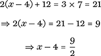
We carry out these four inverse operations in turn on both sides of our equation to yield a sequence of increasingly simple expressions:

and so

the film is Fellini’s .

Our equation (7) is still a simple equation or, as they are more often called, a linear equation. A linear equation is one that can be written in the form ax + b = c, and (7) can be converted to that form for, starting from the 2(x − 4) = 9 stage, we may expand the bracket by the distributive law to obtain 2x − 8 = 9 and this is an equivalent equation, meaning that it is a consequence of and has the same solution as the original. The reason why the term linear is used stems from the general fact that the graph of all points (x, y) such that y= ax + b is a straight line (Figure 3): the line intercepts the y-axis at the point (0, b) and has slope (or gradient)a, meaning that for each unit moved in the positive x direction, we move a units up in the y direction.

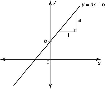
3. Graph of a typical linear function y = ax + b.

It may happen, however, that the unknown x appears more than once in our equation yet it may be possible, using just the laws of algebra, to reduce the equation to the standard linear form. As a more complicated example, let us take

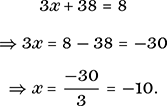
We cannot treat the tangle on the left as the result of a sequence of operations applied to a single instance of x. The first simplification comes about, however, by multiplying both sides by the denominator, 4 − x, as the LHS then becomes simply x + 38 and we have the following upon multiplying out the brackets:

We next add 2x to both sides in order to have only a single term in x. This gives

Simultaneous equations

At what temperature do the Celsius and Fahrenheit scales agree? That is to say, when do the two scales simultaneously give the same value? To answer this we need to know how the scales are calibrated. The Celsius scale is set at 0° at the temperature where water freezes, while 100° is the point where water boils (at sea level). These two temperatures are respectively marked at 32° and 212° on the Fahrenheit scale. If we let y denote temperature in Fahrenheit and x the value in Celsius, then the two are related by an equation of the form y = ax + 32 as when x = 0, y = 32. To find the value of the slope a we note that a rise of 212 − 32) degrees Fahrenheit corresponds to an increase of (100 − 0) degrees Celsius, so that:

For example, if global warming led to an increase in the atmospheric temeperature by 2°C, this would represent an increase of Fahrenheit. However, a Fahrenheit reading (y) is related to a Celsius reading (x) by the linear equation , so that an air temperature of 2°C corresponds to a temperature of 3 ⋅ 6 + 32 = 35 ⋅ 6° F. It is important not to confuse temperature changes with scale readings when discussing such topics!

Returning to our problem, we simultaneously require that y = x, so what we need to find is the point where the two lines that represent these equations cross (Figure 4).

It is natural to substitute y = x into our conversion equation and solve

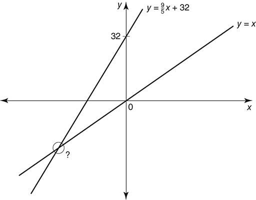
4. Temperature in Celsius and Fahrenheit.

multiplying both sides by the reciprocal, , we extract the required value of x:

Therefore −40° is the unique value where the Celsius and Fahrenheit scales agree.

This is an example of a problem that involves the solution of a pair of simultaneous linear equations, namely

Geometrically, the two equations represent a pair of straight lines and the problem is to find the point where the two lines meet. The points that lie along a particular line in the xy coordinate plane, often known as the Cartesian plane, are those points (x, y) that satisfy an equation of the form ax + by = c, where a, b, and c are fixed numbers that depend on and determine the line in question. Alternatively, we may rearrange this equation if we wish to make y the subject and we obtain the alternative slope–intercept form of the equation:

We therefore turn to the general problem of finding the intersection point of two lines represented by general linear equations. Although only an example, the next problem is fully representative of the general situation, meaning that the way we solve it can be applied to any and all problems of this type. Our two equations are

In our first example we had y = x as our second equation, allowing us to substitute for y immediately. We could take that approach again, make y (or x) the subject of one of the equations, and substitute into the other accordingly. A different tack, though, is based on the idea that we could eliminate one of the variables simply by adding or subtracting the equations if the coefficients of one of the variables were opposites or were equal. In this example this is not the case, but we can get an equivalent pair of equations where this is so by multiplying the first equation throughout by 3 and the second by 2. Doing this, we find we may eliminate x by adding the two equations:

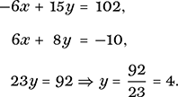
Now we substitute y = 4 into the first equation to give

Therefore the solution to our system of equations is x = −7, y = 4.

This elimination approach (adding and subtracting multiples of equations) is generally a quicker way to find the solution of the system, for it allows us to eliminate a variable using fewer steps than the substitution method. We shall take up an example with more than two unknowns in the final section of this chapter.

Substitution arises from first isolating a variable and then substituting accordingly, thereby eliminating that variable. The value of elimination is that you achieve the same thing while working solely with the coefficients. Matrices, which we introduce in Chapter 7, represent the vehicle for abstracting this process.

Inequalities

In this section we introduce the use and manipulation of inequality signs. Information about unknowns can come in the form of an equality, an equation if you will, or it can arise as a constraint, which can take the form of an inequality such as 2x − 1 ≤ 5. The signs < and ≤ mean less than and less than or equal to, respectively, and of course the signs > and ≥ stand for greater than and greater than or equal to, respectively. Each of these signs points to the smaller quantity in any statement in which it appears. Of course, the simple denial of equality, a ≠ b, is an inequality, but the types of inequality that are most useful in mathematics are the directional inequalities as they often represent upper or lower bounds of quantities of interest and, with some important caveats that will now be explained, may be manipulated in a similar fashion to equalities.

We may be familiar with the meaning of an inequality such as a > b when dealing with positive numbers, but we need to explain its meaning for any numbers, be they positive, negative, or zero. In line with our experience of positive numbers, we shall say quite generally that a > b means that a − b is a positive number. This definition orders the number line in the fashion that you probably take for granted: b < a if b lies to the left of a on the line, so, for example, , and −1 < 0 < 1 are all true statements.

Returning to our inequality 2x − 1 ≤ 5, we can make x the subject of the inequality in the same fashion as used when dealing with an equals sign: in this case we add 1 and then divide by 2 to simplify the constraint to x ≤ 3.

There is, however, one significant complication that arises when dealing with inequalities that is a source of inconvenience and frequent error. Take an inequality such as 2 < 3 and multiply both sides by a negative number, let us say −6. The left and right sides become respectively −12 and −18, and −12 > −18. And so we have another rule: when an inequality is multiplied (or divided) by a negative number, then the direction of the inequality is reversed. For example, let us simplify 4 − 3x ≤ 13. Subtracting 4 from both sides and then dividing through by −3 gives us

This rule is a consequence of our definition. For instance, suppose that a < b and let c < 0. Now, a < b means that b − a is positive, so that c(b − a) is negative, which is to say that cb − ca is negative, so its opposite, ca − cb is positive, which tells us that cb < ca. In conclusion, if a < b and c < 0 then ca > cb, and the direction of the inequality has indeed reversed.

Having cleared that up, it seems that we can continue confidently with our algebraic manipulations. When dealing with an inequality, however, we may wish to multiply both sides by an unknown, x say, but the resulting direction of the inequality depends on the sign of x. When this type of scenario arises we need to be patient and examine the cases that arise separately. We may sometimes, however, avoid multiplying by terms of unknown sign and thereby avoid splitting the problem into separate cases.

For example, suppose we wish to know for what values of x the following inequality holds:

If we now multiply throughout by x + 2, the inequality will change the direction if x < −2, but otherwise will not. Let us instead add 8 to both sides and place the LHS over a common denominator:

A common factor of 3 now appears in the numerator, which we extract and, remembering that , we may cancel to obtain

(8)

A quotient such as we have in (8) will be negative exactly when the numerator and denominator have different signs. A sign change may occur at a point where the term in question takes on the value 0, which is evidently at x = −2 for x + 2 and at for 3x + 5. It is helpful to chart the sign behaviour of each term on a number line.

From Figure 5, we see that the numerator and denominator have the same sign except between the values of −2 and , where x + 2 > 0 but 3x + 5 < 0, and so that then is where our inequality holds: .

Inequalities are used throughout mathematics, often to find bounds of complicated functions in terms of simpler ones. Many useful inequalities stem from the simple observation that a square of a number is never negative. This follows from the fact that the product of two numbers with the same sign is positive. We shall give an instance of this, but first a word about square roots.

For any positive number a, by the square root of a we mean the unique positive number b such that b² = a. This is written as so, for example, . Of course, it is also the case that (−5)² = 25, so every positive number really has two square roots, , although if we speak of the square root, implicitly we mean the positive one. One useful property of square roots is that the square root of a product is equal to the product of the square roots, and, similarly, the square root of a quotient is the quotient of the square roots:

5. Signs of the expressions x + 2 and 3x + 5.

That this is true is a consequence of the commutative law and the fact that two positive numbers are equal if and only if their squares are equal. To verify the first formula, then, we just need to check that the squares of both sides are the same: now, by the very definition of the square root, we have , while

and there is a similar tale for the quotient case. These rules are often used to simplify square roots of numbers that are not perfect squares. For example,

Since the sign √ indicates the non-negative root, it follows that if we begin with a negative number x, then is not x but rather is −x: for example, . The function has a special name: it is called the absolute value function and it has its own notation, |x|. Another way of thinking of |x| is as the distance of x from 0 on the number line, an interpretation which generalizes nicely when we deal with complex numbers, which we shall meet in Chapter 5. Of course |x| is always positive, except when x = 0, as |0| = 0.

The absolute value function is unpopular with just about everyone as, on the one hand, it seems so simple as to be hardly worth mentioning and, on the other hand, it misbehaves algebraically. Just like the square root, it does not behave linearly, meaning that just as it is not generally true that , nor is it true that |a + b| = |a| + |b| (for example, if a = 1 and b = −1, the LHS is 0 while the right-hand side (RHS) is 2).

One rule, however, which is easily verified by looking at cases, is that |ab| = |a| ⋅ |b|; so, for example, we may replace | − 2x| by | − 2| ⋅ |x| = 2|x| in any calculation. In practice, you have to be patient and split a calculation involving absolute values into cases where the object between the absolute value signs is negative and where it is not. It is worth noting, however, that an expression such as |x| ≤ 3 is equivalent to −3 ≤ x ≤ 3 and the latter is more amenable to algebraic manipulation. For example, let us simplify |2x − 1| < 5:

Returning to our search for inequalities based on squares, we introduce the arithmetic mean m of two numbers, a and b, which is what is normally referred to as their average: m = (a + b)/2. If we confine ourselves to non-negative numbers a and b, then the geometric mean g of a and b is defined as . A square with sides of length g has the same area as an a × b rectangle.

For example, if a = 4 and b = 9 then , while . If you experiment with a few examples of your own, you will discover that the arithmetic mean is never less than the geometric. And here is why:

which is just to say that g ≤ m. Moreover, the initial inequality is a strict inequality except when a = b, in which case both means share this common value of a. In every other case, the arithmetic mean exceeds the geometric.

Lincoln Fair problem

As an example that brings together both the notion of inequalities and simultaneous equations, we close this chapter with the following problem that dates back to the 16th century, if not earlier. Twenty people pay twenty pence to visit the Lincoln Fair. If each man pays threepence, each woman tuppence, and each child a halfpenny, how many men, M, women, W, and children, C, went to the fair?

We can take the information given to extract two equations in three unknowns—the first counts people while the second counts pennies:

(9)

Having more unknowns than equations generally means you do not have enough information to solve the problem, or, to be more precise, there is more than one solution. As we have already mentioned, the equation ax + by = c represents a line in the xy plane and, in an analogous way, an equation of the form ax + by + cz = d represents a plane in 3D x, y, z coordinates. Two such planes generally intersect in a line, and so any one of the infinite number of points along that line will have coordinates (x, y, z) that simultaneously satisfy each of the equations of the two planes. Undaunted, we see how far our elimination technique can take us in this problem. Multiplying the first equation by 3 and then subtracting the second equation will at least eliminate the men, giving us

(10)

We can now also express M in terms of C by using our first equation:

When we remove the brackets in this last expression, we must remember to subtract every term inside the brackets (and not just the first one); subtracting the term of course gives . Continuing and rearranging the order of the terms, we infer that

(11)

We have managed to express M and W in terms of C. If we knew no more than the pair of equations (9), we could go no further: we could choose any number for C and determine W and M from C using (10) and (11), and the trio of numbers (C, W, M) that resulted would be a solution to (9); and, what is more, every solution to (9) would arise in this way. We do, however, know more, although the additional information not captured by our simultaneous equations (9) comes in the form of inequalities.

You cannot have fractional or negative people, and so, assuming that there was at least one person of each of the three types, we have the three inequalities C, W, M ≥ 1. There is another more subtle point that is revealed by looking at the second of our two equations in (9): in order that the left-hand side adds up to the whole number 20, the number of children must be even. Hence we may write C = 2A, say, where A is itself a positive integer. Using this and (10) and (11) allows us to write our inequality for W as follows:

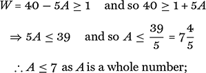
Similarly, M = 3A − 20 ≥ 1 ⇒ 3 A ≥ 21 and so A ≥ 7.

Hence we simultaneously have A ≤ 7 and A ≥ 7, so that A = 7 and therefore C = 2A = 14. There were C = 14 children, and so M = 3A − 20 = 21 − 20 = 1, and W = 40 − 5A = 40 − 35 = 5. Therefore one man, five women, and 14 children went to the Lincoln Fair.

Whenever any system of equations is solved, we may verify the solution by substituting: in this example, putting C = 14, W = 5, and M = 1 into each of our equations in (9) shows that our solution does indeed work. As our reasoning has proved, this is the unique solution to the Lincoln Fair problem provided that we assume there was at least one man, one woman, and one child. Some of the unknowns could, however, be permitted to take on the value 0 without reducing the problem to total nonsense. This would weaken the constraints to C, W, M ≥ 0. If you rework the problem, you find that a second value, A = 8, is now also feasible. Putting A = 8 then gives a second solution: (C, W, M) = (16, 0, 4): 16 children, no women, and four men does, strictly speaking, still work.

There is an entire realm of mathematics, known as linear programming, that is dedicated to solving huge systems of linear equations subject to constraints on the values of the solutions. Our Lincoln Fair problem is a very simple historical instance of this kind of question. This mathematics underpins much of the logistics of modern society, governing operations such as railway and airline schedules while allowing businesses to meet customer demand by running inventories with much less stock stored in warehouses than was required in times past, which represents an enormous and ongoing cost saving. The algebraic ideas of elimination and constraint satisfaction underlie all this. Contemporary society could not function without them operating, behind the scenes, invisibly and flawlessly on behalf of everyone.