Sedimentological Characteristics of the Quaternary Groundwater Aquifer, Northwestern Nile Delta, Egypt

Abstract

A total of 110 sediment samples were collected at various levels during the well drilling. Mechanical analysis of 70 sediment samples was done in order to study the sedimentological and depositional environments of the studied aquifer. Another 40 samples were subjected to X-ray diffraction (XRD) analysis to detect the mineralogical composition of the aquifer sediments. The sedimentary work revealed that the majority of the samples are medium to coarse clayey sand, moderately sorted and coarse skewed. This may support the multi-directional depositional currents. The present-day, wind action influences skin of the sediments. The samples lie within the field of river processes. Mineralogical analysis by X-ray diffractometry revealed that smectite is the most abundant clay mineral, followed by kaolinite, whereas illite is the less abundant clay mineral. The essential carbonate minerals are calcite and dolomite whereas non-carbonate minerals include quartz, feldspar, and hematite.

1 Introduction

Sedimentological studies are of expanding significance in environmental research, especially contamination studies, where past patterns in ecological procedures should be joined with information on current conditions to foresee likely future changes [1]. Sedimentology is a vital branch of geology and its utilization in water resources administration, contamination investigations of subsurface water bodies and depositional condition cannot be over underscored. The presumptions that groundwater is perfect and drilling ought to be done blindly are demonstrations of ignorance and the outcomes far exceed the benefits. Basic sedimentological information should shape some portion of any evaluation of possibly polluted destinations and part of examinations concerning the scattering and catching of contaminants in fluvial frameworks [2]. These information are additionally required for sound ecological administration to guarantee that planning policies are good with common environmental limitations [1].

Sedimentological examination of subsurface borehole sediments is a noteworthy part in groundwater study and aid to predict the depositional condition utilizing fundamental standards of geology [1, 3–5]. The stratigraphy of a landscape assumes an imperative part in groundwater pollution particularly when the aquifer geometry is unconfined [6–8]. When the aquifer is unconfined and shallow, there is a high possibility of contaminants whatever source and kind, particularly when they are near a highly populated area with high anthropogenic effect [9]. Omorogieva and Imasuen [10], Joshua and Oyebanjo [11] estimated that aquifer deposits come from the close surface, igneous outcrops, volcanic and sedimentary rocks. Some of these are effectively disintegrated, though others, particularly the crystalline rocks, are influenced by streams just when adjusted in the surface [12].

It has been perceived that grain-size distribution of granular permeable media influences its hydraulic conductivity [13]. This interrelationship is helpful for the estimation of conductivity properties where coordinate permeability information is inadequate in the beginning times of aquifer investigation. In groundwater hydrology, the learning of soil conductivity is vital for demonstrating the water flow both in the saturated and unsaturated zone, and transportation of water-dissolvable contaminations in the aquifer. The textural properties of an aquifer are all the more effectively acquired, a potential option for evaluating hydraulic conductivity of soils is from grain-distribution [14].

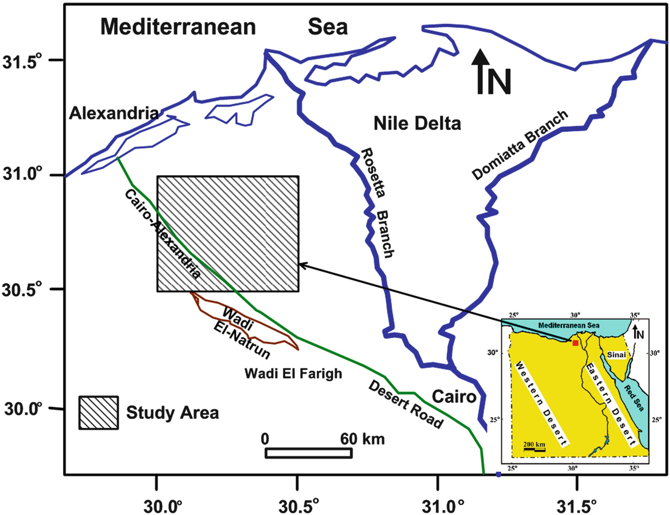
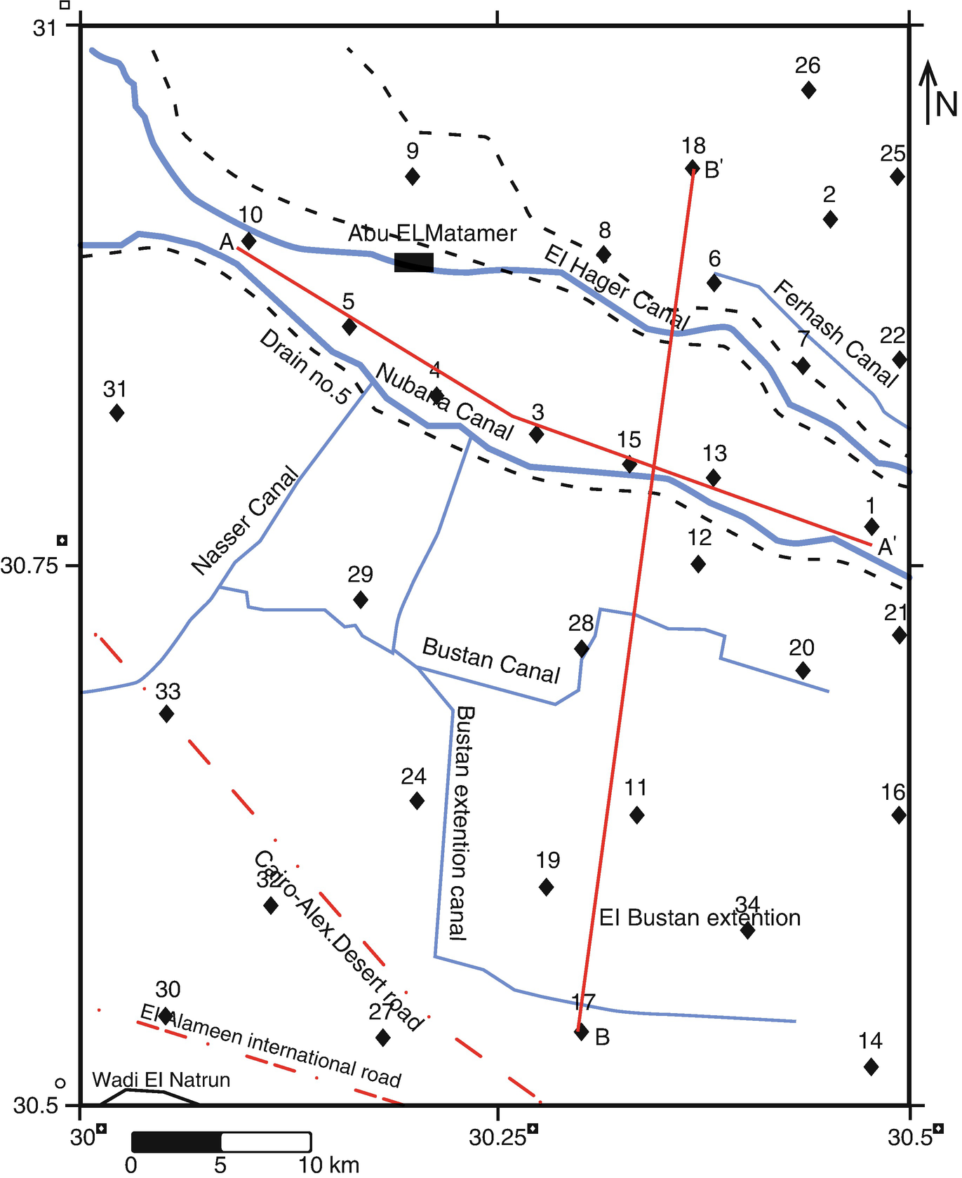
The sedimentary clastic rocks are characterized by high porosity and permeability and forming most of the groundwater aquifers. In the Nile Delta area in general and particularly the study area (Fig. 1), the main aquifer is the Pleistocene which consisted of sand and gravels with clay lenses intercalations. So, the sedimentary formation (i.e., Pleistocene aquifer) analysis for the study area is very important to reveal the aquifer properties as the grain size analyses and mineralogical study. This study deals with the grain size analysis and mineralogical study of the Plio-Pleistocene sediments of the area under consideration.

../images/437178_1_En_153_Chapter/437178_1_En_153_Fig1_HTML.png — Fig. 1
Location map of the study area

2 Study Area

West of the Nile Delta is one of the biggest groundwater territories in northern Egypt. Groundwater potentiality and dispersion are controlled by the geographic location, the sedimentary succession, the geologic structure, and physiographic setting. The study area is situated in the west of the Nile Delta in northern Egypt (Fig. 1). Its geographical boundaries are 30° 30′ and 31° 00′ N and longitudes 30° 00′ and 30° 30′ E. The common territories in this area are north of Wadi El Natrun, El Bustan extension reclamation project, west and east of El Nubaria canal, Abu El Matamir area, and Housh Eissa area.

Many authors studied the stratigraphy of the study area; among them El Fayoumy [15]; Shata et al. [16]; Omara and Sanad [17]; El Ghazawi [18]; Abdel Baki [19] and Abdel Wahab [20]. As disused in Salem and Osman [21, 22], sediments of the study aquifers are of Quaternary (Recent and Pleistocene), Neogene (Pliocene and Miocene), and Oligocene ages (Fig. 2). The Pleistocene aquifer is the most vital aquifer that has a greatest thickness of 300 m to the east to the northeast (Fig. 2a). The Holocene deposits are located in the western part of the investigated area and are composed of eolian sand (4–10 m thick) with calcareous intercalations (Fig. 2b). The Pleistocene aquifer is composed of gravels and sands with thin clay intercalations (Fig. 2b, c). This Quaternary aquifer overlays the clay-rich sediments of Pliocene and Miocene ages (Fig. 2b, c). The Pleistocene aquifer is mostly unconfined but of semiconfined characters at the northern direction where clays cover is predominant. Surface leakages from the watering framework trenches are the principal recharge source for the Pleistocene aquifer [19].

../images/437178_1_En_153_Chapter/437178_1_En_153_Fig2_HTML.png — Fig. 2
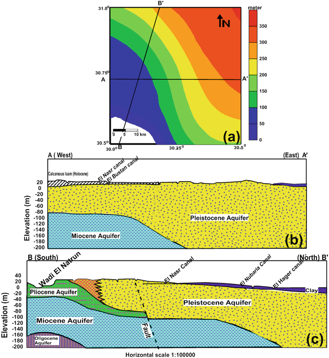
Shows the hydrogeology of the study area. Pleistocene aquifer thicknesses increase to the eastern and northern directions is shown in (a). The hydro-stratigraphic succession of the study area along the cross-sections AA′ and BB′ is shown in (b) and (c), respectively (after [21])

Structures including faults, folds, and unconformities influence the groundwater movement. The West Nile Delta region comprises the northern portion of the great Marmarican Homocline. The strata dip gently to the north and eastward reflecting the effect of the structural elements of the Taphro-geosynclinal basin of the Nile Delta basin [16]. The structural map of the area compiled by different authors is shown in Fig. 3. Major faults with downthrown sides due east have been delineated along the western margin of the Nile Delta. These faults have led, among other geologic features, to the facing of the highly permeable Pleistocene gravel of the Nile Delta opposite to older impermeable sediments to the west. This situation accelerates the subsurface westward flow of Nile water to the older sediments [23]. Two subsurface faults in the area were detected by El Ghazawi [18] comprising El Galala fault (F7) with downthrown to east and displacement reaches about 65 m, and El Nubaria fault (F8) with downthrown also to east (Fig. 3). They are related to the clysmic system during Neogene times. However, the rapid vertical and lateral facies changes of the Quaternary sediments hide this displacement. On the other hand, four probably subsurface faults (F3, F4, F5, and F6) have been detected with downthrown to the Nile Delta [24]. They greatly affect the thickness of the Pleistocene aquifer.

../images/437178_1_En_153_Chapter/437178_1_En_153_Fig3_HTML.png — Fig. 3
Compiled structure map of the study area (after [18, 23, 24])

Wadi El Natrun anticlinal structure trends E 35^° W and extends for about 60 km from El Ralat depression in the north to Beni Salama depression in the south [20]. It is a symmetrical structure affected by parallel and diagonal faults, among them F1 and F2 that led to the formation of the main central depression (Fig. 3). Unconformities are recognized in the area between the Quaternary deposits and Pliocene deposits, where Wadi El Natrun Formation (Early Pliocene) is covered directly by Quaternary clastics, and El Hagif Formation is absent (Late Pliocene) [18].

3 Methodology

The performed working methodology of this work is shown in Fig. 4. Thirty four boreholes were drilled in the study area (Fig. 5). A total of 110 sediment samples were collected at various levels during well drilling. Lithologic log of each well was constructed and then 2D and 3D lithological correlations were performed (Figs. 6 and 7). Mechanical analysis of 70 sediment samples was done to study the sedimentological and depositional environments of the studied aquifer. Results of the grain size analysis were represented in Table 1 and Figs. 8 and 9. The grain size analysis was carried out on the sand fraction using the standard sieving method. Another 40 samples were subjected to X-ray diffraction (XRD) analysis to detect the mineralogical composition of the aquifer sediments. Identified mineralogical compositions for the selected samples are shown in Table 3 and some representative X-Ray Diffractograms are plotted in Fig. 10. The mineralogical analysis was done on bulk samples by X-ray diffraction (XRD) analysis to delineate the clay and non-clay minerals of the sediment.

../images/437178_1_En_153_Chapter/437178_1_En_153_Fig4_HTML.png — Fig. 4
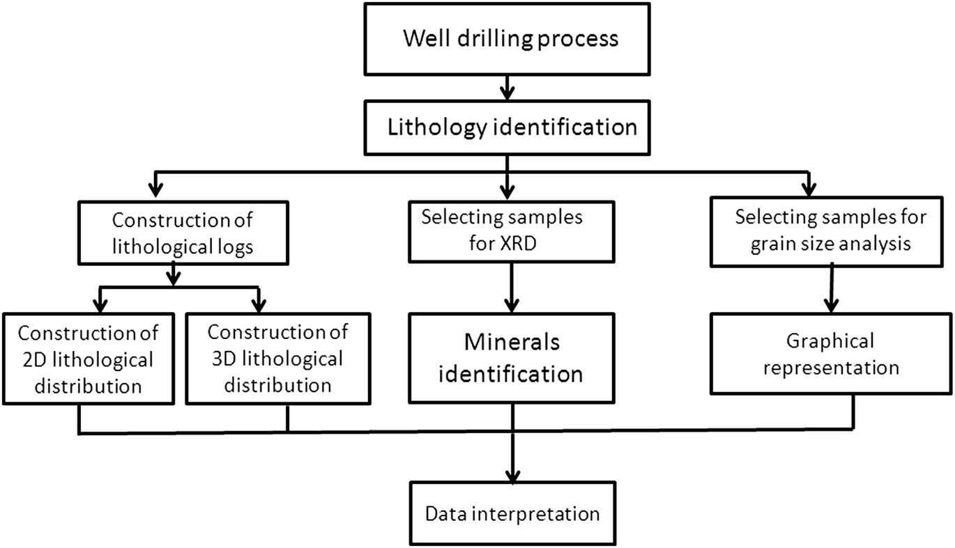
Flowchart shows the working methodology

../images/437178_1_En_153_Chapter/437178_1_En_153_Fig5_HTML.png — Fig. 5
Borehole and the 2D cross-sections location map

../images/437178_1_En_153_Chapter/437178_1_En_153_Fig6_HTML.png — Fig. 6
Vertical lithological distribution along the West-East cross-section (AA′, a) and the South-North cross-section (BB′, b)

../images/437178_1_En_153_Chapter/437178_1_En_153_Fig7_HTML.png — Fig. 7
3D lithology models of the study area

Table 1

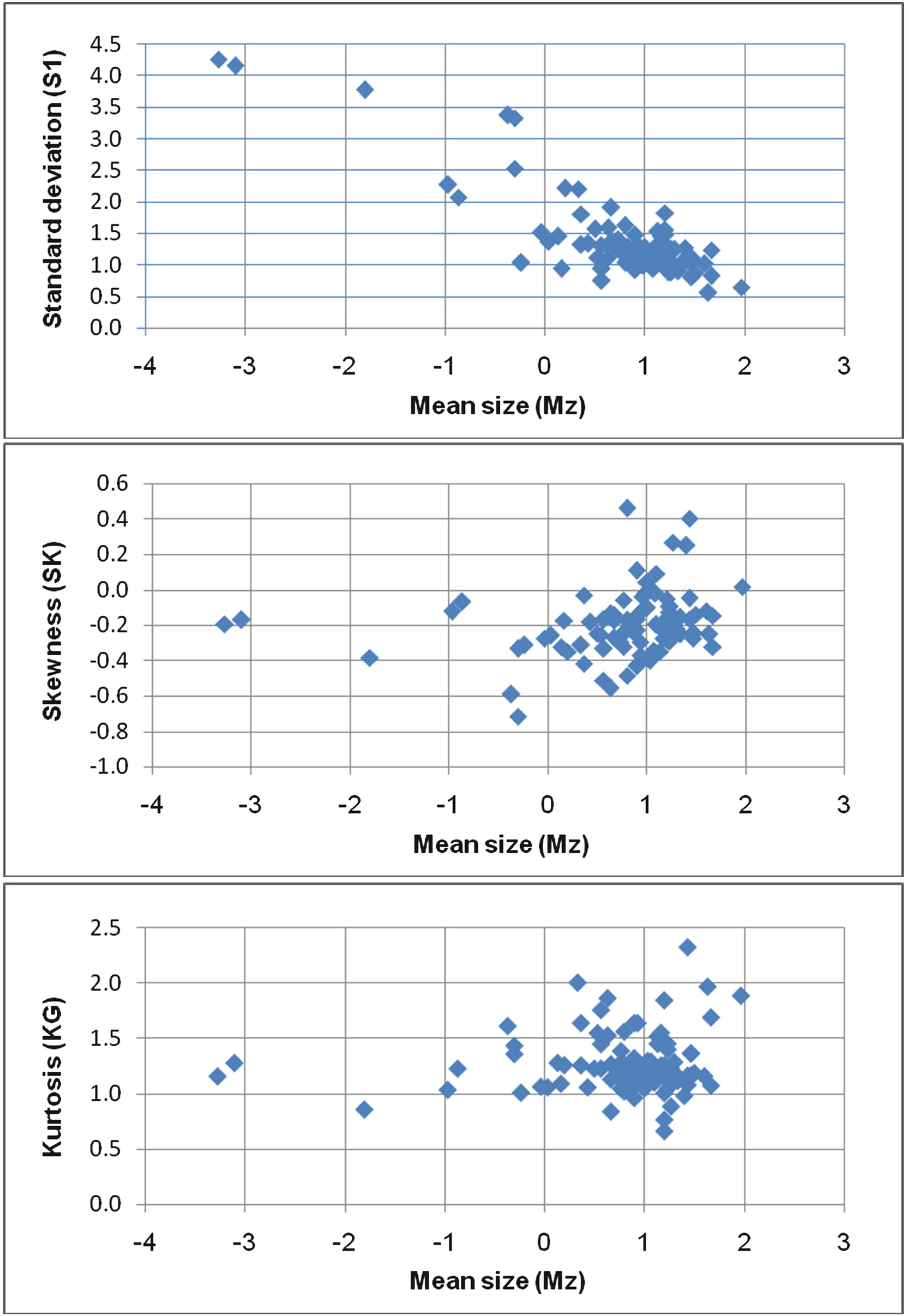
Statistical grain size parameters of the collected samples

Well no.	Sample depth (m)	Md	Mz	S_I	SK_I	KG_I
1	1	1.10	1.43	1.07	0.40	2.32
	5	0.80	−0.37	3.37	−0.59	1.61
	10	0.60	0.20	2.21	−0.35	1.26
	15	0.50	0.33	2.21	−0.31	2.00
	25	0.90	0.67	1.91	−0.27	1.27
	35	−2.80	−3.27	4.27	−0.19	1.16
2	40	0.70	0.57	0.75	−0.33	1.76
	45	1.05	1.08	0.93	−0.02	1.19
	55	0.60	0.43	1.34	−0.18	1.06
	60	1.70	1.67	0.83	−0.14	1.69
	70	0.95	0.98	0.98	−0.02	1.19
	75	0.80	0.53	1.12	−0.25	1.55
	90	1.30	1.13	1.07	−0.35	1.45
	100	0.70	0.63	1.12	−0.14	1.53
	125	1.30	1.27	0.96	−0.15	1.19
	140	1.40	1.33	0.90	−0.16	1.12
3	20	1.10	0.93	1.31	−0.37	1.64
	28	1.00	1.00	1.03	−0.10	1.20
	48	0.90	0.77	1.27	−0.24	1.39
4	20	1.30	0.90	1.24	−0.42	1.07
	25	1.00	0.77	1.29	−0.32	1.13
	30	1.30	1.03	1.14	−0.40	1.23
	35	1.30	1.10	1.08	−0.36	1.20
	40	1.30	1.03	1.13	−0.39	1.30
	50	1.00	0.73	1.40	−0.30	1.18
	55	0.30	0.03	1.37	−0.26	1.06
	60	1.00	0.90	1.10	−0.23	1.20
	65	1.30	1.03	1.13	−0.39	1.20
	70	1.20	0.80	1.62	−0.48	1.56
	80	0.90	0.77	1.31	−0.24	1.28
	90	1.50	1.43	1.11	−0.17	1.08
	100	0.30	0.80	1.04	0.46	1.26
	110	1.30	1.20	0.96	−0.24	1.01
	130	1.50	1.33	0.99	−0.25	1.16
5	1	−0.70	−0.87	2.07	−0.07	1.23
	100	0.90	0.80	1.18	−0.17	1.02
	110	0.80	0.67	1.36	−0.17	1.13
6	10	0.90	0.57	0.94	−0.51	1.23
	30	0.70	0.50	1.57	−0.25	1.23
	50	−1.00	−1.80	3.78	−0.38	0.86
	80	0.30	0.17	0.93	−0.17	1.09
	120	1.00	0.90	1.16	−0.17	1.32
	150	1.00	0.97	1.01	−0.04	1.10
7	27	1.00	−0.30	3.33	−0.72	1.43
	35	1.20	1.10	1.29	−0.20	1.20
	43	1.00	0.93	1.08	−0.13	1.11
	48	0.10	−0.23	1.04	−0.31	1.01
	97	1.70	1.63	0.56	−0.25	1.97
	106	0.80	0.67	1.26	−0.14	0.84
7	120	1.20	0.93	1.25	−0.29	1.26
7	125	0.70	0.57	1.30	−0.17	1.45
8	22	1.40	1.20	1.48	−0.24	0.77
8	133	1.40	1.20	1.24	−0.28	0.67
9	0	1.00	1.27	1.24	0.27	0.89
	40	1.00	1.40	1.28	0.25	0.98
	70	1.40	1.27	0.90	−0.20	1.23
	75	1.60	1.47	0.80	−0.24	1.37
	80	0.90	1.03	1.07	0.00	1.27
	85	1.60	1.60	1.02	−0.12	1.16
	102	1.90	1.97	0.65	0.02	1.89
11	12	−2.60	−3.10	4.16	−0.17	1.28
	25	1.00	0.87	1.05	−0.24	1.13
	27	1.60	1.47	1.06	−0.25	1.17
	30	1.00	1.10	1.01	0.09	1.10
	35	1.40	1.27	0.88	−0.19	1.09
	45	1.20	0.63	1.58	−0.56	1.86
	55	−1.00	−0.97	2.28	−0.12	1.04
	60	0.40	0.13	1.46	−0.32	1.28
12	4	1.40	1.23	1.10	−0.29	1.40
	13	1.60	1.50	0.86	−0.14	1.19
	30	0.80	0.77	1.20	−0.06	1.05
	44	1.30	1.17	1.45	−0.28	1.55
13	10	1.20	1.20	1.21	−0.05	1.26
	30	1.30	1.17	1.30	−0.23	1.26
	40	1.30	1.07	1.10	−0.34	1.29
	50	1.10	1.13	1.53	−0.21	1.52
	60	1.40	1.23	1.02	−0.26	1.45
	120	1.30	1.23	0.88	−0.09	1.19
	135	1.00	0.83	1.29	−0.19	1.13
14	4	1.30	1.20	1.83	−0.16	1.17
	10	1.80	1.67	1.24	−0.32	1.08
	30	1.6	1.47	1.11	−0.28	1.37
14	85	0.80	0.37	1.81	−0.42	1.64
14	15	1.20	1.20	1.55	−0.23	1.84
15	65	0.20	−0.30	2.53	−0.33	1.36
	75	1.40	1.43	1.14	−0.05	1.17
	80	1.30	1.23	1.27	−0.12	1.05
	85	0.80	0.90	1.23	0.11	0.96
	90	1.40	1.30	1.24	−0.22	1.29
	120	0.90	0.90	0.92	−0.15	1.15
	130	1.20	0.90	1.47	−0.43	1.64
	140	0.90	1.00	1.30	0.04	1.05
	150	0.40	0.37	1.33	−0.03	1.26
	155	0.20	−0.03	1.51	−0.27	1.07

Mz mean size, Md median size, σl standard deviation, Sk skewness, KG kurtosis

../images/437178_1_En_153_Chapter/437178_1_En_153_Fig8_HTML.png — Fig. 8
The relationship between mean size (Mz) on one hand and standard deviation (σ1), skewness (SK), and kurtosis (KG) on the other hand of the Pleistocene sediments

../images/437178_1_En_153_Chapter/437178_1_En_153_Fig9a_HTML.png — Fig. 9
Bivariate plots of the statistical grain-size parameters for the studied sediments (a and b boundaries after [25]; c after [26]). (d) Boundary after Friedman [27], (e) and (f) after Moiola and Weiser [28]

../images/437178_1_En_153_Chapter/437178_1_En_153_Fig9b_HTML.png — Fig. 9
Bivariate plots of the statistical grain-size parameters for the studied sediments (a and b boundaries after [25]; c after [26]). (d) Boundary after Friedman [27], (e) and (f) after Moiola and Weiser [28]

../images/437178_1_En_153_Chapter/437178_1_En_153_Fig10_HTML.png — Fig. 10
X-Ray Diffractograms of some selected samples in the area. From up to down, these diffractograms are for samples 8 (well 14), 30 (well 9), 36 (well 12), 56 (well 9) and 90 (well 8). Horizontal axis represents two-theta (degree) and the vertical axis represents the relative peak intensity (counts) for each diffractogram

4 Result and Discussion

4.1 Lithological Correlation

The samples from different wells drilled in the area (Fig. 5) are distributed overall the area at various depths (Table 1). The cross-sections AA′ and BB′ (EW and SN, respectively) were established (Fig. 6) to show the vertical and lateral lithology changes. These sections revealed that the sediments of the area are formed of fine to medium sand, gravels, and clay lenses at different levels. Cross-section AA′ (Fig. 6a) extends from E-W direction and contains seven lithology wells [1, 6, 19, 27, 29–31]. The general cross-section composition is sand from fine to coarse size. The sand and gravel sediments which are considered as an ideal groundwater aquifer are recorded in wells 12, 4, 5, and 10. Intercalations of some clay lenses are recorded all over this cross-section. These lenses might affect the level and quality of the groundwater in the investigated aquifer.

Cross-section BB′ contains six wells [23, 27, 32–35] (Fig. 6b) and shows that, the ground level is decreased toward the northern direction. It also indicates that the sand thickness increased to the central part and decreased to the southern and northern directions. In contrast, the number and thickness of the clay lenses increased to the southern and northern directions. Also, the constructed 3D models (Fig. 7) show the lithology variations as represented from AA′ and BB′ cross-sections in all directions. The 3D model shows the increasing of sand thickness toward the central part. Increasing in number and thickness of the clay lenses toward south, north and deeper zones led to decrease in sand thickness.

4.2 Granulometric Analysis

The granulometric study of sediment is an important textural parameter which measures the energy of the depositional environment. Both the friable and semi-friable samples from different wells were selected for the grain size analysis by sieving method. The statistical parameters of Folk and Ward’s [31] were calculated from the grain size data. The data were then plotted on the cumulative curves.

The grain-size parameters include graphic mean (Mz), median size (Md), inclusive graphic standard deviation (Si), skewness (SK) and kurtosis (KG). The diagrams proposed by Stewart [25], Friedman [26, 27], Moiola and Weiser [28], and Mason and Folk [35] have been applied to recognize the depositional environments of the sediments. The data of grain size distribution of the analyzed samples were plotted on cumulative curves, and the calculated parameters are shown in Table 1, and the summary of the grain size parameters is shown in Table 2 .

Table 2

Summary of the grain size parameters of the collected samples

Parameter	Phi value (φ)		Description
Mz	Range	−3.27 to 1.97	Medium pebbles to medium sand
Mz	Average	−0.6	Very coarse sand
Md	Range	−2.8 to 1.9	Fine pebbles to medium sand
Md	Average	−0.4	Very coarse sand
σ1	Range	0.56–4.27	Medium well sorted to extreme poorly sorted
σ1	Average	2.45	Very poorly sorted
SK	Range	−0.72 to 0.46	Strongly coarse to strongly fine skewed
SK	Average	−0.13	Coarse skewed
KG	Range	0.67–2.32	Platykurtic to Leptokurtic
KG	Average	1.5	Leptokurtic

4.2.1 Univarient Grain Size Parameters

The mean size of sediments is controlled by the average energy distribution in the deposition media, the initial size and the source material [31, 36, 37]. It can be determined by using Eq. (1):

$\mathrm{Mz}=\left({\phi}_{16}+{\phi}_{50}+{\phi}_{84}\right)/3$

(1)

in which Mz is the mean size and ϕ ₁₆, ϕ _50, and ϕ ₈₄ represent the size at 16, 50, and 84% of the sample by weight, respectively.

The mean size value of the Pleistocene samples (Table 2) ranges from −3.27 to 1.97 Φ (medium pebbles to medium sand) with an average value of −0.6 Φ (very coarse sand). The values of mean size fluctuate frequently reflecting the change of the depositing medium.

Grain sorting depends on the sediment source, grain size, and depositional regime [31]. The inclusive graphic standard deviation (σ) for the studied sediment varies from 0.56 to 4.27 Φ (medium well sorted to extreme poorly sorted) with an average value of 2.45 Φ (very poorly sorted). It can be calculated by using Eq. (2):

$\sigma =\left({\phi}_{84}-{\phi}_{16}\right)/4+\left({\phi}_{95}-{\phi}_5\right)/6.6$

(2)

where ϕ ₁₆, ϕ _84, ϕ _5, and ϕ ₉₅ represent the size at 16, 84, 5, and 95% of the sample by weight, respectively.

Skewness (SK) is a measure of symmetry of grain size distribution, and it is very useful descriptive term for the depositional processes of the sediment. The values of (SK) in these samples range from −0.72 to 0.46 Φ (strongly coarse sorted to strongly fine skewed), with an average value of −0.26 Φ (coarse skewed). It is calculated by [31], using Eq. (3):

$\mathrm{SK}=\left\{\left({\phi}_{16}+{\phi}_{84}-2{\phi}_{50}\right)/2\left({\phi}_{84}-{\phi}_{16}\right)\right\}+\left\{\left({\phi}_5+{\phi}_{95}-2{\phi}_{50}\right)/2\left({\phi}_{95}-{\phi}_5\right)\right\}$

(3)

According to [31], Kurtosis (KG) is a measure for the peakedness of the grain-size distribution. The obtained values of (KG) range from 0.67 to 2.32 Φ (platykurtic to leptokurtic) with a mean value of 1.5 Φ (leptokurtic). The graphic Kurtosis is given by Eq. (4):

$\mathrm{KG}=\left({\phi}_{95}-{\phi}_5\right)/2.44\left({\phi}_{75}-{\phi}_{25}\right)$

(4)

where ϕ ₇₅ and ϕ ₂₅ represent the size at 75 and 25% of the sample by weight, respectively.

4.2.2 Bivariate Grain-Size Parameters

The bivariate plots between grain-size parameters are very useful in discriminating the depositional environments of rock [31]. The relationships between the calculated statistical parameters are discussed below, and their bivariate plots are given in Fig. 8.

The scatter plot diagram of the mean size versus the inclusive graphic standard deviation (Fig. 8a) shows that the majority of the samples are scattered around the field of moderately sorted, except some poorly sorted and well sorted samples. It further indicates that the decrease in the mean size of sediment is associated with better sorting.

Skewness has successfully been used by Mason and Folk [35], Friedman [14] and Moiola and Weiser [28] to differentiate between various environments of deposition. Strong skewed samples reflect zones of mixing environments [38]. The plot of skewness versus mean size shows that the majority of the samples are coarsely skewed (Fig. 8b). Such behavior may support the multi-directional depositional currents.

The relationship between mean size and kurtosis (Fig. 8c) further indicates that the present sand is leptokurtic. The leptokurtic character corresponds to what Mason and Folk [35] termed “aeolin flat.” This term does not mean that the sediments were deposited by aeolian agent but means that the present day skin of the sediments is influenced by wind action [30]. This explains the more pronounced leptokurtic characters of the studied samples.

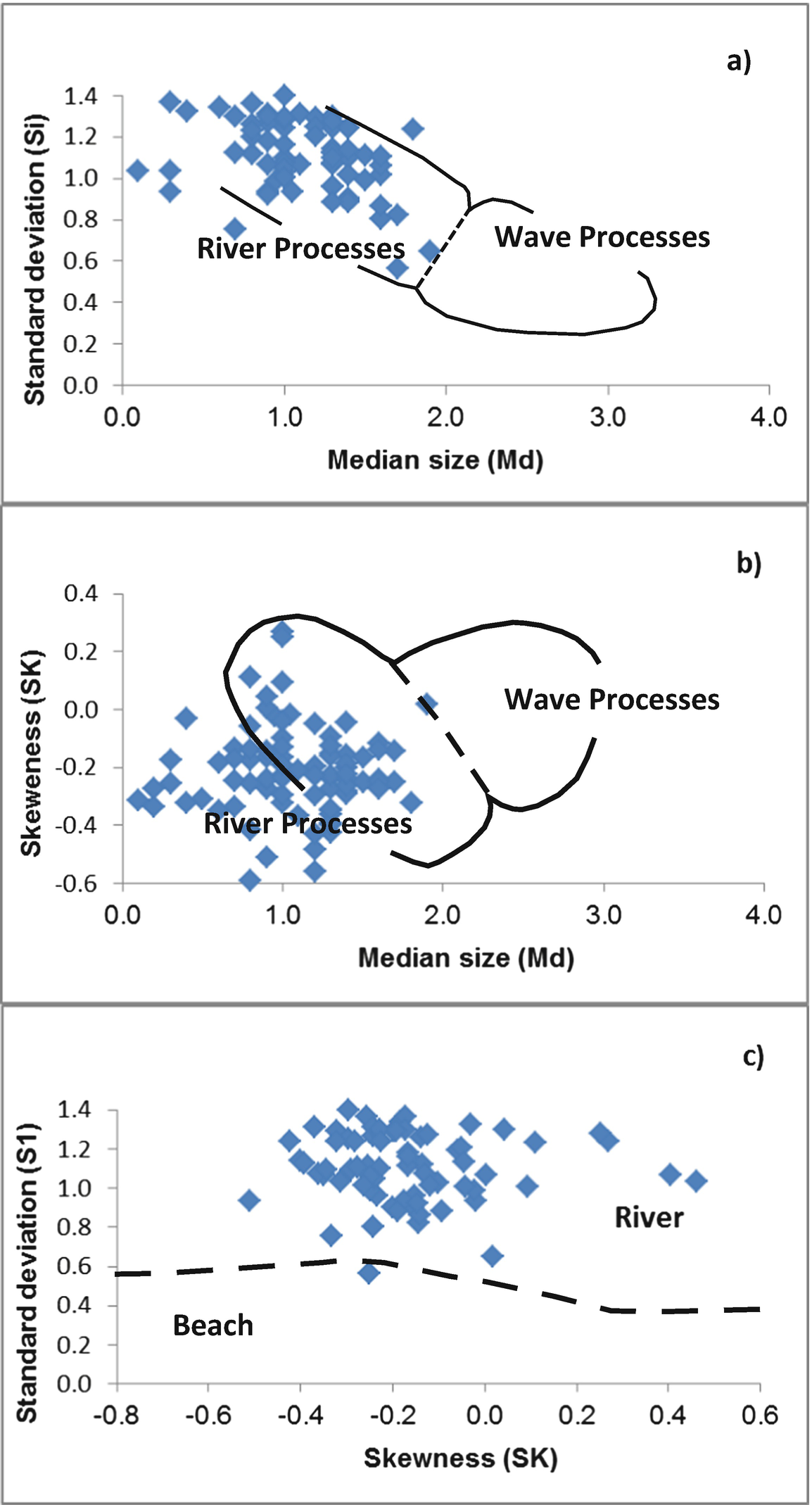
Stewart [25] suggested that the plot of median diameters versus each of standard deviation and skewness is important to differentiate between river and wave processes. The plot of sorting vs. median diameter (Fig. 9a, b) indicates that the total samples lie within the field of river processes. Also, the plot of skewness versus median diameter shows that the total samples lie within the same field.

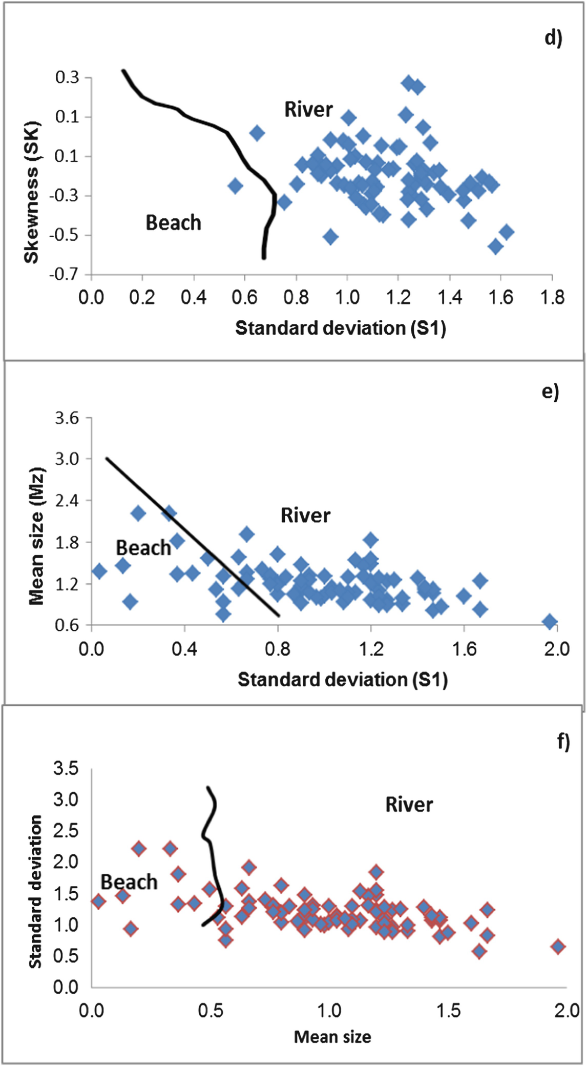
The plot of skewness versus standard deviation [26] shows the studied samples are distributed in the field of fluvial environments. The total samples belong to the river sands (Fig. 9c, d). The discriminating fields of Friedman [27] show the total samples are distributed within the river processes.

Moiola and Weiser [28] used various combinations of Folk and Ward’s [31] textural parameters for differentiation between different environments. The plot of standard deviation versus mean diameters (Fig. 9e, f) shows that the most samples are distributed within the river processes, while 18% of the total samples lie within the beach environment.

4.3 Mineralogical Analysis

The mineralogical analysis was carried out on some selected bulk samples using X-ray diffractometry. The data of semi-quantitative determination of clay minerals are given in Table 3. X-Ray Diffractogram of the fine fraction of the studied sediments suggests that the clay mineral associations are dominated by smectite, kaolinite, and illite (see Fig. 10).

Table 3

X-ray diffraction data of the collected bulk samples

Well no.	Sample depth	Clay minerals			Non-clay minerals
Well no.	Sample depth	Smectite	Illite	Kaolinite	Quartz	Feldspars	Calcite	Hematite	Dolomite
1	45	24.0	2.1	12.5	38.5	12.5	8.3	2.1	0
	50	5.4	1.8	8.1	12.6	4.5	63.1	4.5	0
	80	23.7	7.9	11.8	28.9	9.2	13.2	5.3	0
	85	17.3	5.1	7.1	45.9	9.2	10.2	5.1	0
2	6	30.6	3.3	16.5	20.7	9.9	12.4	0.0	6.6
2	17	30.5	3.8	16.8	21.4	13.0	11.5	3.1	0
3	10	34.3	3.7	13.9	23.1	11.1	9.3	4.6	0
3	37	40.7	5.5	11.0	18.7	11.0	9.9	3.3	0
4	5	5.9	5.9	16.1	16.9	5.9	47.5	1.7	0
	10	16.5	12.1	5.5	38.5	11.0	11.0	5.5	0
	15	27.9	6.3	9.0	31.5	10.8	14.4	0.0	0
	40	25.8	6.5	12.9	30.3	10.3	10.3	3.9	0
5	75	33.3	0.0	16.2	18.9	14.4	14.4	2.7	0
5	90	22.4	5.1	12.2	45.9	7.1	5.1	2.0	0
7	45	15.6	6.5	9.1	37.7	15.6	10.4	5.2	0
	87	29.3	5.4	10.9	32.6	10.9	5.4	5.4	0
	96	11.8	2.7	11.8	25.5	10.9	28.2	9.1	0
	98	36.3	4.9	27.5	15.7	9.8	2.9	2.9	0
	104	20.7	3.7	17.1	24.4	14.6	12.2	7.3	0
	107	15.1	5.4	9.7	39.8	17.2	7.5	5.4	0
	118	16.9	7.0	11.3	23.9	14.1	18.3	8.5	0
	130	26.7	4.0	21.3	20.0	18.7	0.0	9.3	0
8	55	32.7	5.1	22.4	25.5	0.0	10.2	4.1	0
	90	29.8	3.5	14.2	25.5	14.2	9.2	3.5	0
	135	10.8	4.3	11.8	48.4	21.5	0.0	3.2	0
9	5	29.7	5.4	12.2	27.0	10.8	9.5	5.4	0
	10	18.2	3.6	7.3	38.2	25.5	0.0	7.3	0
	30	16.0	5.6	7.2	45.6	12.0	9.6	4.0	0
	56	19.9	4.0	8.5	41.5	15.3	8.5	2.3	0
	73	13.3	3.1	5.1	58.2	10.2	7.1	3.1	0
12	15	38.5	3.3	13.2	24.2	9.9	11.0	0.0	0
12	36	38.3	0.0	13.8	28.7	10.6	8.5	0.0	0
13	80	23.5	5.9	17.6	36.8	16.2	0.0	0.0	0
	100	36.3	4.4	14.3	24.2	8.8	8.8	3.3	0
	102	23.4	4.7	12.5	31.3	17.2	10.9	0.0	0
14	8	41.1	4.0	11.3	17.9	7.9	14.6	3.3	0
14	30	30.0	7.3	9.1	24.5	13.6	12.7	2.7	0
Average		24.7	4.7	12.7	30	12	12.1	3.8	0.2

4.3.1 Clay Minerals

Smectite is the most abundant clay mineral in the studied sediments (Fig. 10). Its average value reaches up to 24%. The highest value (41.1%) is recorded in the north-central part of the area at 8 m depth, while the lowest value (5.4%) is obtained in the central part at 50 m depth. Smectite may be formed under authigenic and/or detrital conditions [39, 40]. Authigenic smectite may be formed in both continental and marine environments. Authigenic smectites formed in the continental aqueous sedimentary environment are essentially restricted to saline alkaline lakes and characterize the unusual water chemistries that may develop in these settings [32].

In the marine environment, authigenic smectites may be originated from the alteration of volcanics, mixing of ocean waters and plumes of hydrothermal fluid or halmrolysis (submarine weathering) and direct precipitation on the sea floor [41]. Detrital smectites may be formed under exogenous conditions chiefly upon weathering of basic igneous rocks, in alkaline medium. They also may be formed by secondary detrital degraded lattices (mica or chlorite), where their inter-sheet K⁺ or Mg⁺⁺ ions are replaced by water molecules [42].

Kaolinite is the second abundant clay mineral encountered in the studied sediments. The average value of kaolinite reaches 12.6%. The highest value (22.4%) is obtained in the northern part at 55 m depth, while the lowest value (5.1%) at 73 m depth in the central part. Kaolinite usually has a detrital origin, although authigenic kaolinite may also be precipitated from circulating groundwaters that are supersaturated with alumina and silica [33]. Typically, kaolinite develops in continental areas subjected to strong chemical weathering. It usually favors moderately warm to humid and well-drained acidic continental areas, where the rate of precipitation is much higher than the evaporation rate. Under these conditions, chemically soluble elements are preferentially removed leaving residual silica and alumina which are involved in the formation of kaolinite [43]. As kaolinite formation requires acidic leaching conditions, it cannot be formed under marine settings [44].

In the alkaline marine environment, there is no leaching, and the water contains a good deal of dissolved calcium. These environmental conditions favor the formation of smectite rather than kaolinite. A study of weathering processes indicates that kaolinite does not form calcareous parent material until all the carbonate has been removed. This kaolinite is likely to be transported to the marine environment by rivers and/or by the wind. It may also have a diagenetic origin. Velde [45] has shown that kaolinite is generally abundant in the early diagenesis, but as depth and maturity of rocks increase, kaolinite becomes less abundant.

Robert and Kennett [46] linked kaolinite abundances to increased precipitation and deposition during high stand of sea level. The great relief of drainage basins, established during low stand of sea level, favors the formation of kaolinite, especially during warm and humid conditions. However, Robert and Chamley [47] found no significant correlation between the abundances of kaolinite and sea level fluctuations.

Kaolinite is a typical low latitude clay mineral [48] and its concentration increases in tropical regions. Millot [43] assumed that kaolinite is dominant in fluviomarine and lacustrine deposits. Kaolinite formation requires strong leaching environment, an acid reaction medium and the presence of aluminum silicates [40]. The formation of kaolinite requires a favorable climate and an environment of high depleted cations other than Al and Si. Perrin [49] considered kaolinite as the most stable clay mineral that does not undergo appreciable change during transportation. However, diagenetic alteration of kaolinite in the marine environment has been noted by Biscaye [29].

Illite is the less abundant clay mineral encountered in the studied sediments. Its average value reaches up to 24%. Illite has a continental origin according to age determination [34]. It is formed by the weathering or partial hydrolysis of muscovite. Thus, it occurs often in soils derived from the weathering of mica-schist, gneisses, acid and medium igneous rocks in association with smectite and other minerals. Weaver [50] indicated that illite could often be formed from smectite in marine environments.

Diagenetic alteration of montmorillonite and kaolinite into illite generally occurs where sedimentation rates are low and time is also important for the chemical interaction between seawater and clay minerals [51]. Illitization of kaolinite is mentioned by Rumeau and Kulbicki [52]. Potassium and magnesium in seawater would be expected to promote the formation of the more stable clay minerals at the expense of the less stable ones.

4.3.2 Non-clay Minerals

The mineralogical examination has been carried out on some selected carbonate rocks using XRD technique. The data of bulk samples (Table 3) show that the essential carbonate minerals are calcite and rarely dolomite whereas noncarbonate minerals include quartz, feldspar, and hematite. The essential carbonate minerals in the studied samples are calcite and rare dolomite. These minerals are detected by their basal reflection at 3.04A and 2.88A, respectively, and their abundances are calculated by measuring peak height above the background. Calcite is the most common carbonate mineral in the studied samples. It is easily identified by the X-ray diffraction technique where the major peak appears at (3.04A). The average percent of calcite reaches about 11.8%. Dolomite is recorded only in two samples. Its identification is aided by X-ray diffraction technique, where the major peak appears at (2.88A). The average percent of dolomite reaches about 5.9%.

Quartz, feldspar, and hematite are detected in the studied samples. These minerals were detected by their basal reflections at 3.4A, 3.25A, and 2.69A, respectively, and their abundances are calculated by measuring the peak heights above the background. The most common detrital minerals in the samples are quartz and feldspar. Quartz is one of the most common detrital minerals in the samples. It is identified by X-ray diffraction technique where the major peak appears at (3.35A). Table 3 shows that the percentage of quartz ranges from 0 to 62% with a mean value of 10.8%. Feldspar is the second abundant detrital mineral in the samples as its chemical stability is lower than that of quartz. Its mean value is 11.8%. Hematite is the lowest mineral in the studied samples, and it is identified by X-ray diffraction where the major peak appears at (2.69A), its average value is 3.7%.

5 Conclusions

This study gave basic information for the future groundwater dynamics and water–rock interaction research in the study area. The grain size analysis data could help for hydraulic conductivity calculations, and the mineralogical description could answer many questions about the change in groundwater salinity and chemistry along the flow system.

The sedimentological study revealed that

1.
The main composition of the aquifer in the area is medium sand to medium pebbles, poorly sorted with clay intercalations.
2.
The majority of sediments belong to river sands and river processes with multi-directional depositional currents.
3.
The main clay minerals in the intercalated clay lenses of the aquifer are smectite and kaolinite. The essential carbonate minerals include calcite and dolomite whereas noncarbonate minerals are represented by quartz, feldspar, hematite, and gypsum.

6 Recommendations

Lithological, grain size, and mineralogical analysis of the clastic sediments help to explain the water hydrodynamic and salinity behavior in an aquifer. Therefore the result of this work might be used for future groundwater investigation in the study area.

Acknowledgments

The authors are grateful to Tanta University for the financial support offered during the course of this research work. The authors thank the editor Prof. Dr. Abdelazim Negm for his constructive remarks.

References

1.
Brandly E, David M (1993) Implication of sedimetological studies for environment and management: examples from fluvial systems in North Queensland and West Australia. Sediment Geol 85(1–4):235–252
2.
Imasuen OI, Omorogieva OM, Nwokoloh NJ (2016) Grain size and heavy mineral analyses of two boreholes in recent to miocene aquifer in benin formation. Niger J Technol 35:979–986Crossref
3.
Nwajide CSA (2006) Guide for geological field trip to Anambra and related sedimentary basins in southeastern. University of Nigeria, Nsukka, p 28
4.
Suzuki T (1975) Heavy minerals composition of the recent sediments in 3 different environments. In: Geological survey of Japan part, vol 1, p 501
5.
Tawari GS (2008) Variation of heavy minerals in different lithofacies and Geomorphic Units of Ganga – Yamuna River near their confluence at Allahabad, Uttar Pradesh. Geol Soc India 1:133–140
6.
Akpoborie I (2011) Aspect of the hydrology of the western Niger Delta wetlands: groundwater conditions in the Neogene deposits of the Ndokwa area. Afr Geosci Rev 18:25–36
7.
Onyeobi TUS, Akujieze CN (2014) Characterization of soil and sediment parameters of Jisike-Izombe Upper aquifer system for assessment of potential of groundwater pollution. J Appl Sci Environ Manag 18:674–683
8.
Oteze GE (2011) Water supply, groundwater and flood control in Benin City. In: Presented at the NMGS, Benin chapter sensitization workshop on water resources management and its implications in Benin City, Mar 22
9.
Isikhuemen MI, Omorogieva OM (2015) Hydrogeochemical and biophysical characterization of groundwater in Eastern Nigeria; a case study of Onisha and Environ. Niger J Technol 34Crossref
10.
Omorogieva OM, Imasuen OI (2016) Factors contributing to the concentration of heavy metals in stream sediment along Ikpoba river tributary in Oluku (Upstream) to Ikpoba River Dam (Downstream) and their implication. Niger J Appl Sci 34:187–193
11.
Joshua EO, Oyebanjo OA (2010) Grain-size and heavy metals mineral analysis of river Osun sediments. Aust J Basic Appl Sci 4:498–501
12.
Mahavir S (2001) Heavy mineral assemblage of the pinjor formation of the Northwestern Himalaya and its significance in deciphering the provenance of the sediments. J Geol 54:65–87
13.
Freeze RA, Cherry JA (1979) Groundwater. Prentice Hall, Englewood Cliffs
14.
Rosas J, Lopez O, Missimer TM, Dehwah AHA, Sesler K, Coulibaly K (2014) Hydraulic conductivity and grain size distribution: comparison of methods for different sedimentary depositional environments. Groundwater 52:399–413Crossref
15.
El Fayoumy IF (1964) Geology of groundwater supplies in Wadi El-Natrun area. MSc thesis, Faculty of Science, Cairo University
16.
Shata AA, El Fayoumy IF, Tamer M (1970) Geology, hydrogeology and soil of Wadi El-Natrun-Maryut agriculture project. Int. Rep., Desert Institute, Cairo, p 19
17.
Omara SM, Sanad S (1975) Rock stratigraphy and structural features of the area between Wadi El-Natrun and Moghra depression, western desert, Egypt. Geol Jb B16:45–73
18.
El Ghazawi MM (1982) Geological studies of the Quaternary-Neogene aquifers in the area northwest Nile Delta. MSc thesis, Al-Azhar University, Cairo
19.
Abdel Baki AA (1983) Hydrogeological and hydrochemical studies on the area west of Rosette branch and south of El-Nasr Canal. PhD thesis, Faculty of Science, Ain Shams University, Cairo
20.
Abdel Wahab S (1999) Hydrogeological and isotope assessment of groundwater in Wadi El-Natrum and Sadat city, Egypt. MSc thesis, Faculty of Science, Ain Shams University
21.
Salem ZE, Osman MO (2016) Shallow subsurface temperature in the environs of El-Nubaria canal, northwestern Nile Delta of Egypt: mplications for monitoring groundwater flow system. Environ Earth Sci 75:1241. https://doi.org/10.1007/s12665-016-6046-y Crossref
22.
Salem ZE, Osman OM (2017) Use of major ions to evaluate the hydrogeochemistry of groundwater influenced by reclamation and seawater intrusion, West Nile Delta, Egypt. Environ Sci Pollut Res 24:3675–3704. https://doi.org/10.1007/s11356-016-8056-4 Crossref
23.
El Shazly EM, Abdel-Hady MA, El-Ghawaby MA, El Kassas IA, Khawasil SM, El Shazly MM, Sanad S (1975) Geological interpretation of landsat satellite images for west Nile delta area, Egypt. Remote sensing research project, Academy of Scientific Research Technology, Egypt
24.
Mabrouk MA (1978) Electrical prospecting on the groundwater in the area west of Cairo-Alexandria desert road (between Wadi El-Natron and El-Nasr Canal). MSc thesis, Faculty of Science, Ain Shams University, Cairo
25.
Stewart HB (1958) Sedimentary reflections of depositional environment in San Miguel lagoon, Baja California, Mexico. Bull Am Assoc Petrol Geol 42:2567–2618
26.
Friedman GM (1961) Distinction between dune, beach and river sands from their textural characteristics. J Sediment Petrol 31:514–529
27.
Friedman GM (1967) Dynamic processes and statically parameters compared for size frequency distribution of beach and river sands. J Sediment Petrol 37:327–345Crossref
28.
Moiola RJ, Weiser D (1968) Textural parameters and evaluation. J Sediment Petrol 38:45–53
29.
Biscaye PE (1965) Mineralogy and sedimentation of recent deep sea clay in the Atlantic ocean and adjacent seas and oceans. Geol Soc Am Bull 76:803–831Crossref
30.
El Hinnawi EE, Kabesh ML, Zahran I (1973) Mineralogy and chemistry of Nubian sandstone from the central Eastern Desert of Egypt. N Jb Miner Abh 118:211–234
31.
Folk RL, Ward WC (1957) Brazos River bar, a study in the significance of grain size parameters. J Sediment Petrol 27:3–26Crossref
32.
Chamley H (1989) Clay sedimentology. Springer, Berlin, p 623Crossref
33.
Hendriks F (1985) Upper Cretaceous to Lower Tertiary sedimentary environments and clay mineral associations in the Kharga Oasis area (Egypt). N Jb Geol Paläont Mh 10:579–591
34.
Hurley PM, Heezen BC, Pinson WH, Fairbairn HW (1963) K-Ar age values in pelagic sediments of the north Atlantic. Geochim Cosmochim Acta 27:393–399Crossref
35.
Mason CC, Folk RL (1958) Differentiation of beach, dune and aeolian flat environments by size analysis. J Sediment Petrol 28:211–226
36.
Pettijohn FJ, Potter PE, Siever R (1987) Sand and sandstone, 2nd edn. Springer, New York, p 553Crossref
37.
Sahu WD (1964) Depositional mechanisms of clastic deposition. Am Assoc Petrol Geol Bull 34:73–83
38.
Inman DL (1952) Measure for describing the size distribution of sediments. J Sediment Petrol 22:124–145
39.
Keller WD (1970) Environmental aspect of clay minerals. J Sediment Petrol 40:788–813
40.
Weaver CE (1958) Geologic interpretation of argillaceous sediments. Bull AAPG 42:254–309
41.
Lewis WD, McConchie D (1994) Practical sedimentology. Chapman and Hall, New York, p 190
42.
Musa GA (1985) Sedimentological and micropaleontological studies on Tariff well northeast Nile Delta, Egypt. Unpublished MSc thesis, Faculty of Science, Tanta University
43.
Millot C (1970) Geology of clays. Springer, Berlin, p 429Crossref
44.
Keller WD (1982) Kaoline a most diverse rock in genesis, texture, physical properties and uses. Geol Soc Am Bull 93:27–36Crossref
45.
Velde B (1995) Compaction and diagenesis. In: Velde B (ed) Origin and mineralogy of clays: clays and the environment. Springer, New York, pp 220–246Crossref
46.
Robert C, Kennett JP (1992) Paleocene and Eocene kaolinite distribution in south Atlantic and southern oceanic Antaractic climate and paleoanographic implication. Mar Geol 103:99–110Crossref
47.
Robert C, Chamley H (1991) Development of early Eocene climates as inferred from clay mineral variation in oceanic sediments. Glob Planet Chang 89:315–331Crossref
48.
Rateev MA, Gorbunova ZN, Lisitzin AP, Nosov GL (1969) The distribution of clay mineral in the oceans. Sedimentology 13:21–43Crossref
49.
Perrin RMS (1971) The clay mineralogy of British sediments. Mineralogical Society, London, p 406
50.
Weaver CE (1956) The distribution and identification of mixed layer clays in sedimentary rocks. Am Mineral 14:202–221
51.
Grim RE, Diet RS, Bradly WF (1949) Clay mineral composition of some sediment from the Pacific Ocean of the California coast and the Gulf of California. Geol Soc Am Bull 60:1785–1808Crossref
52.
Rumeau JL, Kulbicki G (1969) Evolution des mineraux agileux dans les dolomites etles calcaries du cretace superieur de lar platforme d’ Aquitaine Intern. In: Clay Conf. 2nd, pp 103–117