1 Introduction
Limitations of water resources are the main problem to achieve the main target of constructing new settlements and land reclamation projects for sustainable development in Egypt. Great attention is paid by different Egyptian authorities for that purpose to overcome the overpopulation crisis and construct new agricultural areas. In this respect, priorities are given to the West Nile Delta area, which is considered as a promising region due to its distinct location, mild weather, easy accessibility, and the availability of water supplies. Accordingly, new desert settlements are established, e.g., South El-Tahrir, El-Sadat city, El-Nubariya, and El-Bustan pilot areas, in addition to many villages and farms.
An adequate supply of freshwater is one of the prerequisites for every type of developmental programs. On the other hand, water conservation is very important because usable water is not an unlimited resource. As water supplies dwindle, water shortages in many areas of the world constitute a major problem for both agriculture and nations. Agriculture consumes more than 80% of the water used annually in several countries, where the water is the most important need in farming, and its deficiency commonly limits plant growth.
Groundwater is the main source for domestic, industrial, and agriculture uses in most of the newly reclaimed areas in the west Nile Delta region [1]. Geophysics, especially geoelectric techniques, has been successfully used to detect the freshwater/saltwater interface in coastal aquifers [2]. Resistivity surveys are often used to search for groundwater in both porous and fissured media (e.g., [3, 4]). The methods provide detailed information about the geometry, source, and amount of contamination [5]. For these purposes, the present research is planned in order to address and evaluate the hydrogeological regime in the area of the West Nile Delta using geoelectrical and electromagnetic methods.
2 Location of the Study Area
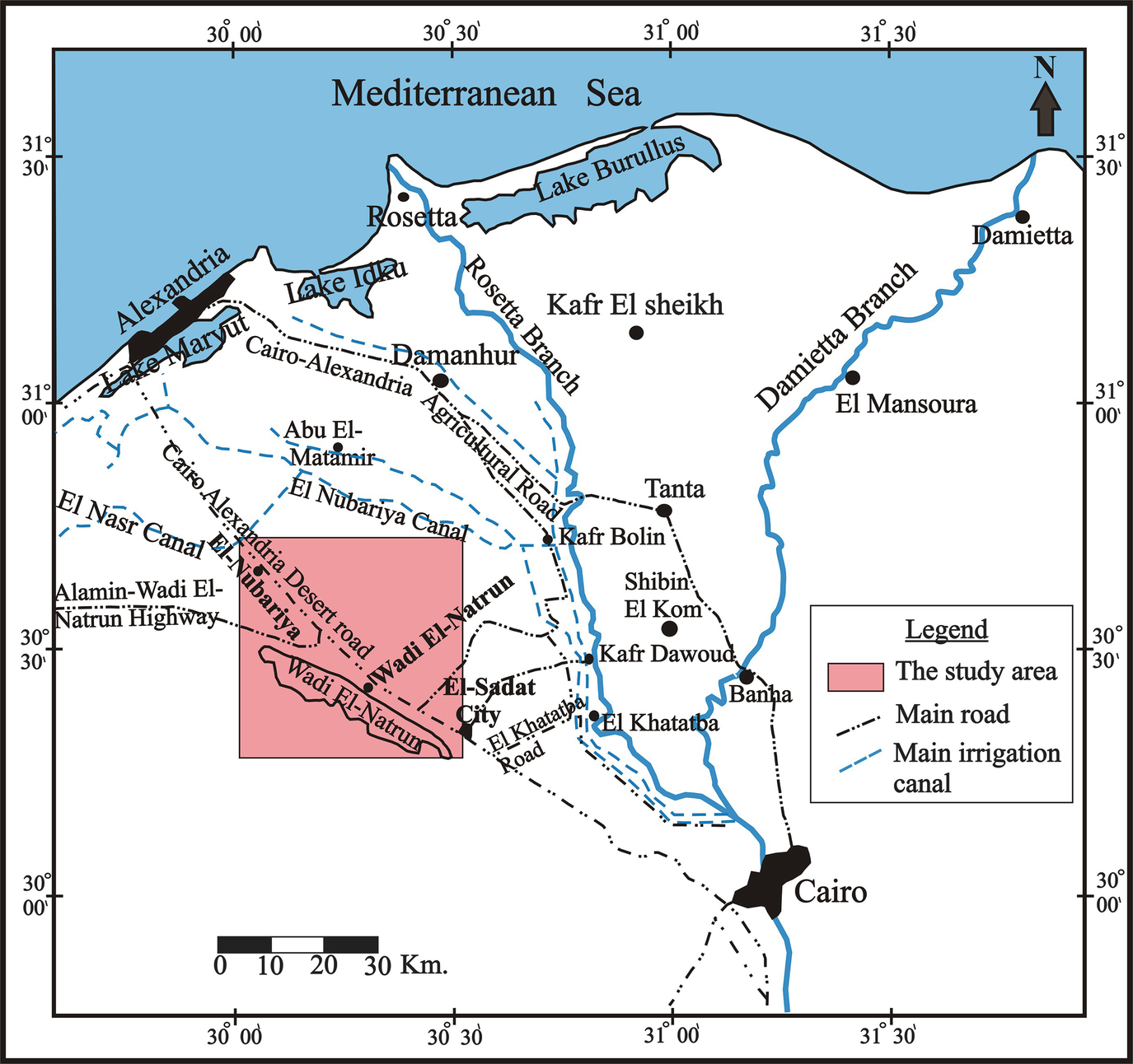
Location map of the study area
3 Geomorphological and Geological Setting
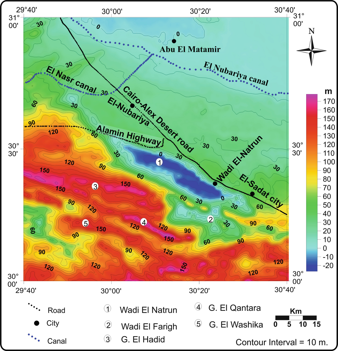
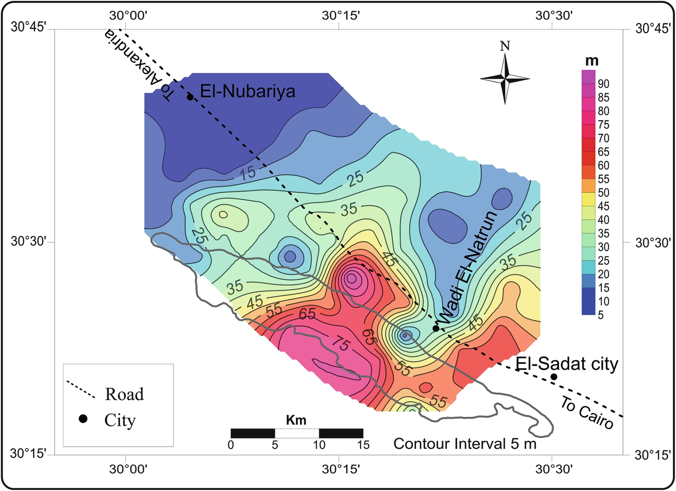
Topographic contour map of the study area (Extracted from GTOPO30 DEM (digital elevation model))
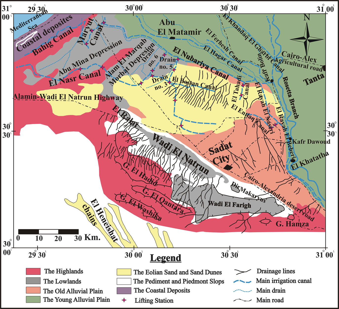
Detailed geomorphologic map characterized by landforms of the study area and its environs (Reproduced after [19])
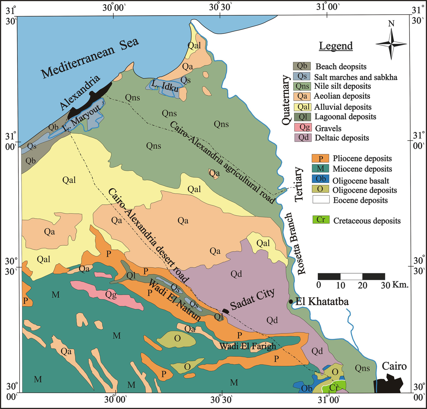
Geological map of the area west of Nile Delta (Reproduced after [28])
Sahara Wadi El-Natrun well, Western Desert, Egypt [9]
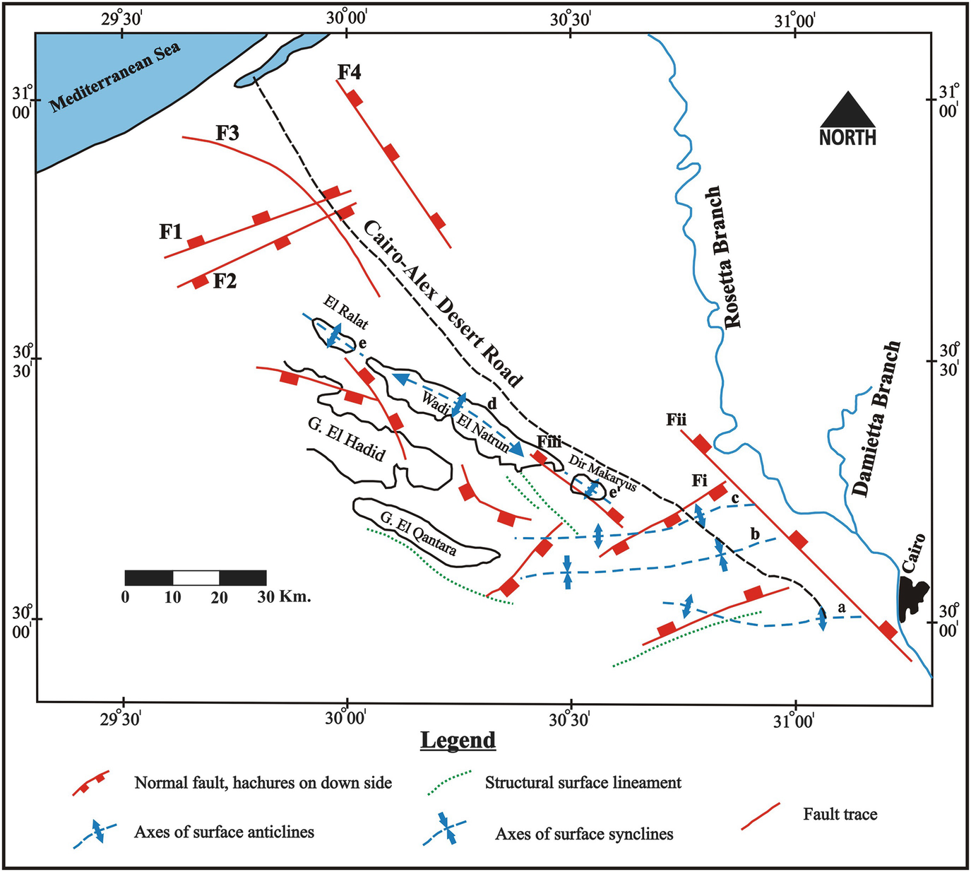
4 Structure and Tectonics
- 1.The NW-SE trending faults: These faults have high displacement.
- (a)
A fault (Fii) runs approximately parallel to the western edge of the Nile Delta [24].
- (b)
A fault (Fiii) runs mostly tangential to the lakes of Wadi El-Natrun with a maximum displacement of about 200 m [31].
- (c)
A fault is transversing the area between Wadi El-Natrun and Gabel El-Hadid with a maximum displacement of about 120 m [12].
- (d)
El Marbat fault (F3) with downthrown of about 50 m due east [33].
- (e)
El-Nubariya fault (F4) running parallel to El Marbat fault with its downthrown side eastward [15].
- (a)
- 2.The NE-SW trending faults:
- (a)
The Rossa fault affects the area between Wadi El-Natrun and Abu Roash and has a length of about 100 km and vertical displacement of about 1 km, with its downthrown side to the north [9].
- (b)
A fault (Fi) lies to the southeast of Wadi El-Natrun and extends to the edge of Rosetta branch.
- (c)
Alam Shaltot fault (F1) to the north of El-Ralat depression with its downthrown side toward the north.
- (d)
A fault (F2) lies to the south of Alam Shaltot fault with a downthrown to the south.
- (a)
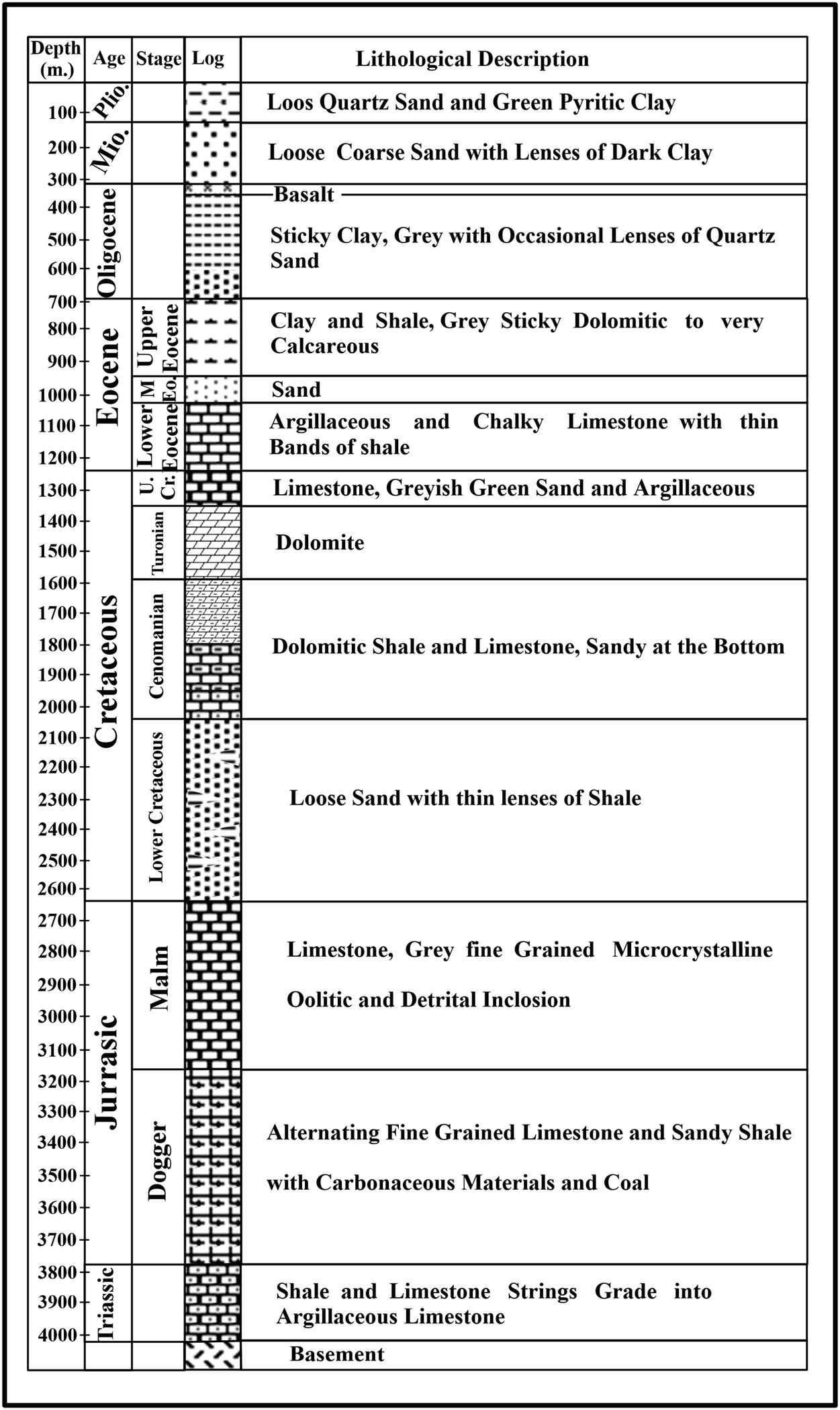
5 Geological History
During the Triassic time, a period of uplift and erosion was recorded where continental conditions prevailed which explain the absence of the Triassic deposits in the area.
The main sea transgression occurred in the study area during the Jurassic producing a great section of marine deposits composed of shaley limestone and dolomites.
Erosion and humid conditions were prevailed during the Lower Cretaceous leading to the deposition of a section of Nubian sandstone strata under continental conditions, while during the Upper Cretaceous period, the study area was subjected to subsidence associated with sea transgression resulting in the deposition of limestone, dolomite, and shale.
The marine transgression was still prevailing during the Eocene times where thick limestone beds were deposited. Also, another regression phase had started during the Late Eocene. Consequently, shallow marine facies (calcareous shale and clay) are characterizing this period.
The Oligocene period is characterized by main terrestrial conditions and the occurrence of a long period of rising and erosion. However, a restricted shallow marine environment is expected in Early Oligocene times, and at the end of Oligocene, volcanic activities dominated.
The Miocene period is characterized by semiarid climatic conditions and the deposition of fluviomarine beds (Moghra Formation) with a gradual subsidence after a long period of rising, erosion, and volcanic activity. Moreover, the surface developed into different morphotectonic features such as Wadi El-Farigh anticline ridge. At the end of Miocene, the initial formation of the River Nile took place (Eonile). Also, epeirogenic movements occurred toward the western part of the Mediterranean Sea during the Miocene times. This was followed by a sea regression, and consequently the lowering of the water level of the Nile producing the Miocene deltaic plains.
A local sea ingression into the Nile Delta and Wadi El-Natrun took place during the Early Pliocene. Consequently, a large marine gulf was developed occupying this area resulting in the deposition of a thick succession of pyritic clay forming aquiclude beds. The gulf was characterized from the south by freshwater tributaries, followed by the deposition of shallow marine limy facies in the Late Pliocene.
In Early Pleistocene times, the prevalence of wet climatic conditions and alluvium filled Abu Mina and El Marbat depressions with gravels and sand brought from the Nile as well as from the tableland. This was followed by lowering of the Nile water level and formation of the old deltaic gravelly plains. The drainage system, particularly on the highlands, was created as a result of the extensive wet climatic conditions.
During the Holocene, landscape took most of its present shape, which is represented by the sand dunes and sand sheets in addition to the formation of lakes in Wadi El-Natrun. The prevalence of the present aridity led to the development of crust layer. The Nile water deposited the young deltaic sediments in floodplains where these soils constitute the most fertile land of Egypt.
6 Hydrogeological Aspects
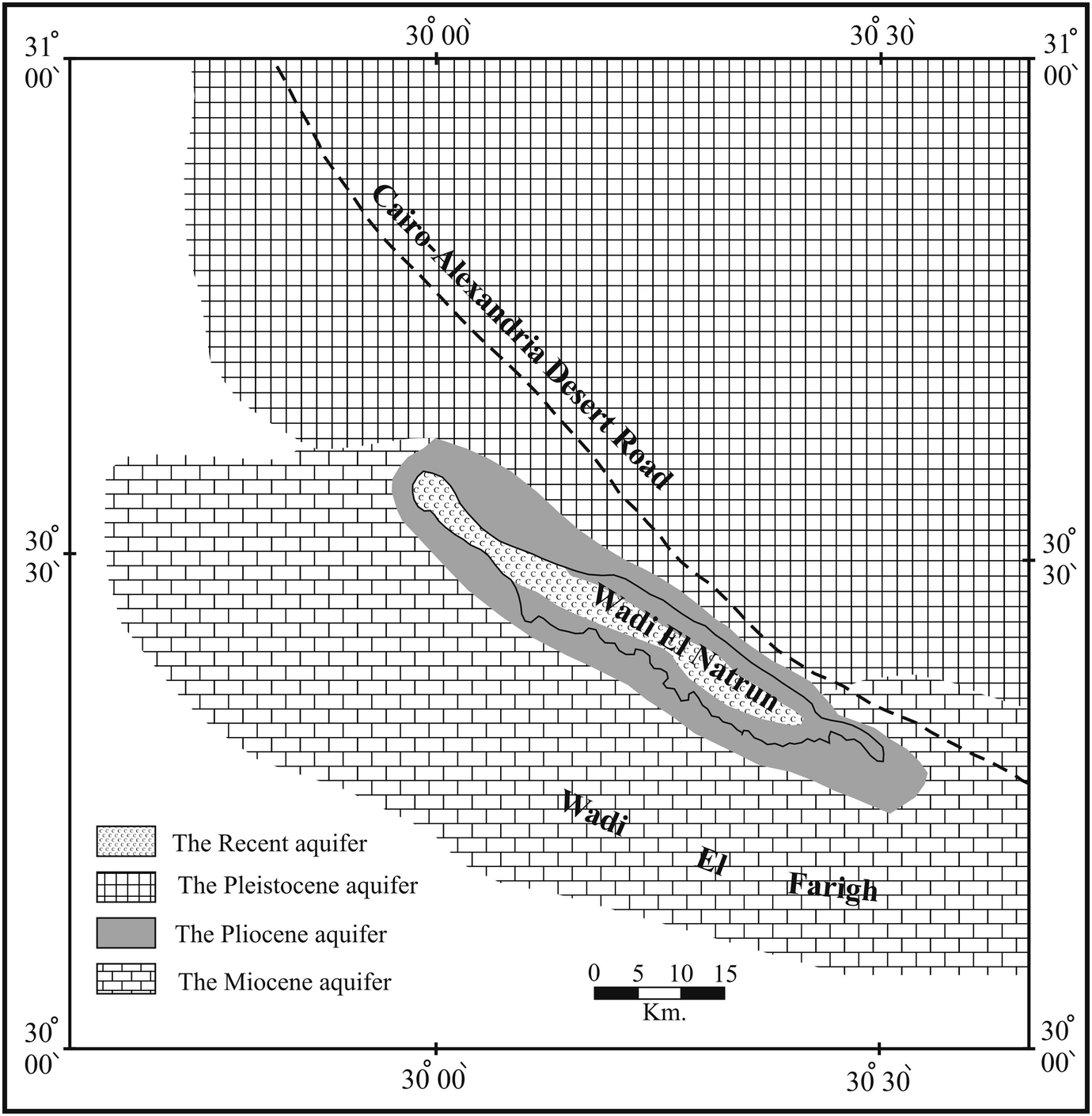
Distribution of shallow aquifers in the study area and its vicinities (Compiled after [16])
6.1 Recent Aquifer
It is detected at Wadi El-Natrun depression and mainly composed of sandy deposits with calcareous intercalations of eolian fillings. This aquifer is considered partial feeder for the salt lakes of Wadi El-Natrun.
6.2 Pleistocene Aquifer
Pleistocene aquifer occupies the major portion of the study area where it is composed of Nile sands and gravels intercalated with thin clay lenses. The depth to groundwater of this aquifer is close to the ground near El-Nubariya canal and increases to the south.
6.3 Pliocene Aquifer
This aquifer dominates the area of Wadi El-Natrun and El-Ralat depressions. It is mainly composed of clay facies with interbeds of water-bearing sandy layers. The Pliocene aquifer sediments can be divided into two horizons [39]. The upper one is composed of loose sand and sandstone having a thickness of about 15 m where the groundwater is existing under semi-confined condition due to the presence of sandy clay layers at its top. Meanwhile, the lower one is composed of sandy facies and has a thickness varying from 1 to 10 m. The groundwater is found under confined condition due to the presence of a thick clay bed between the two horizons.
6.4 Miocene Aquifer
The Miocene aquifer (Moghra Formation aquifer) covers a wide portion in Wadi El-Farigh and west of Wadi El-Natrun to the south and southwest of the study area. It is mainly composed of coarse sands and sandy clay deposits, which rest on the Oligocene basaltic sheets.
7 Background Geophysical Literature
The study area and its surroundings have been subjected to some previous studies; Abdel Baki [16] classified the aquifers in the area west of Nile Delta including the study area into four items: Recent aquifer, Pleistocene aquifer, Pliocene aquifer, and Miocene aquifer. Gomaa [18] compared the hydrogeological and hydrogeochemical properties of the different aquifers west of Nile Delta and found that all the reservoirs are recharged from the Nile Delta Quaternary reservoir. Diab et al. [40] carried out a geoelectric survey (15 VESes with AB/2 ranging from 1 to 300 m) in the north of El-Hamra Lake in the main Wadi El-Natrun depression. The study aimed to interpret the phenomena of the flow up of the freshwater spring in the very saltwater of El-Hamra Lake. They found that the area is affected by inferred horstal structural feature extending into the lake. This horst faulting system brings permeable water-bearing formation against the impervious clay bed holding up the freshwater along the fault plane in the form of a faulting spring. Depending on the hydrochemical analysis of different water samples collected from the spring and the surrounding wells, they declared that the freshwater of El-Hamra spring is feeded from the Miocene artisan aquifer. Abdel Salam [41] found that the aquifers in Wadi El-Natrun area are recharged from the surface water system, El Rayah El Naseri, El Rayah El Beheri, El-Nubariya canal, and El Nasr canal, besides the recharge from the Miocene reservoir of Wadi El-Farigh area. He also confirmed the hydraulic connection between the different aquifers in Wadi El-Natrun area. Using 43 vertical electrical soundings, Abd El-Gawad and Ammar [42] indicated that the Pliocene aquifer is the main aquifer in Wadi El-Natrun area where the water-bearing formation consists of sand layers with clay intercalations and the groundwater exists under confined to semi-confined conditions. This aquifer has a maximum thickness that reaches 200 m which increases to the north and east. The depth to this aquifer ranges between 2 and 24 m. Mansour [43] carried out 35 vertical electrical soundings in the area north of El-Nubariya city and found that the main aquifer is the Pleistocene aquifer where its thickness varies from 14 to 58 m which increases in the east and southwest direction. This aquifer is composed mainly of sand and in some localities of clayey sand or silty sand. The groundwater exists under unconfined or semi-confined conditions. He also concluded that the salinity of the groundwater varies from 600 ppm in the east and southeast and 3,900 ppm (brackish type) in the south. Massoud et al. [44] executed VES and TEM data measurements at 24 stations along three profiles in El-Sadat city. They mentioned that there are two aquifer systems in the area. The shallow Pleistocene aquifer consists of sand and gravel saturated with freshwater and exhibits large thickness varying from 171 to 218 m and depth range of 6–36 m. The deep Pliocene aquifer is composed of clay and sand and shows low resistivity values. Sharaky et al. [1] studied the hydrochemical characteristics of groundwater of western Nile Delta aquifers. They found that the salinity content varies greatly from 430 mg/L (freshwater) to 24,407 mg/L (saline water) with an average of 2,705 mg/L (brackish water). Freshwater is mainly concentrated in the central-eastern part, close to Rosetta branch, indicating that the aquifer is mainly recharged by the infiltration from irrigation network and excess of irrigation water through the upper clay layer. The salinity increases gradually north- and westwards due to seawater intrusion and mixing with the Miocene aquifer, respectively.
8 Hydrogeological Mapping Using VES and TEM Techniques
Electrical resistivity and electromagnetic methods are well known in exploration geophysics and commonly applied in near-surface applications. Electrical resistivity is one of the most useful techniques applied to groundwater studies because the resistivity of rock is very sensitive to its water saturation. Similarly, EM techniques have been particularly succeeded in groundwater exploration and in the mapping of groundwater contamination and saltwater/freshwater interfaces [45–47].
The geoelectric and electromagnetic field surveys give knowledge about the subsurface and structural geology of the studied area; an identification of geometry and extent of the aquifer, some information about the groundwater quality, and a good identification about the lithology of the subsurface formations. Therefore, money, effort, and time can be saved through the reduction of the number of drilled boreholes [48]. Also, a geoelectrical method is considered to be the most promising and most suitable method for groundwater prospecting [49–51]. Although the apparent resistivity values could be considered a direct criterion for the presence or absence of groundwater, general information about water salinity could be also detected, since these values are inversely proportional to the salinity factor [52].
- 1.
The recent sophistication of instruments worldwide.
- 2.
The field data acquisition is quicker compared to DC methods.
- 3.
The method does not need large spreading like resistivity method and does not need a large number of people for field work.
- 4.
The method does not need direct contact with the earth because we use a loop of wire on the surface of the earth, so if we have different conditions for working by resistivity, we can easily use the electromagnetic method.
Electromagnetic methods have been extensively developed and adapted over the past three decades for the lateral and vertical mapping of resistivity variations [53, 54]. The depth of investigation of an electromagnetic field depends upon its frequency and the electrical conductivity of the medium, through which it is propagating. The depth of penetration thus increases as both the frequency of the electromagnetic field and the conductivity of the ground decrease.
8.1 Electrical Resistivity of Rocks
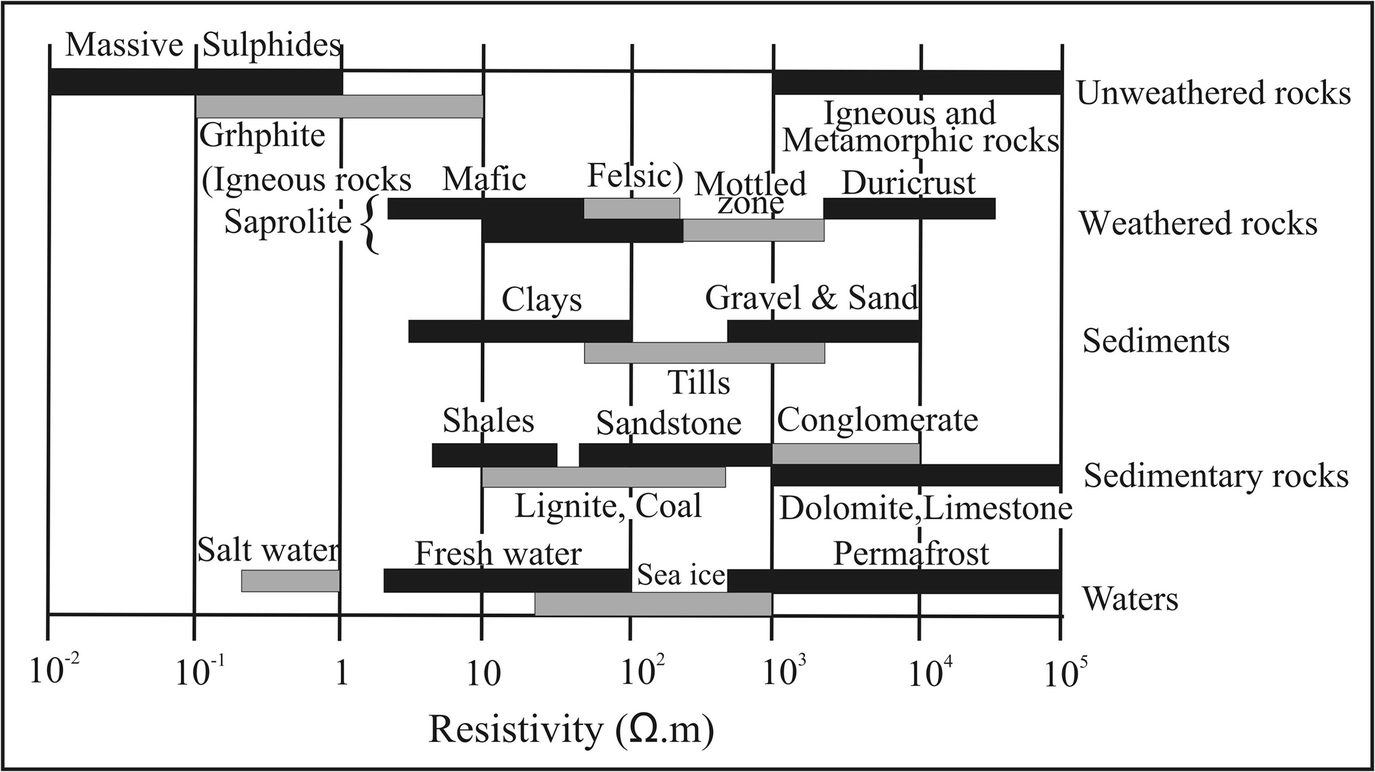
Electrical resistivity of different rocks and materials [59]
However, there are overlaps in the resistivity values of the different types of rocks and soils. This overlap due to the resistivity is a function of the quality and amount of water, porosity, and fractures in these rocks. The resistivity of the freshwater varies from less than 10 to 100 Ω m depending on the salinity of this water. Freshwater has much lower ion concentrations and lower conductivity. The resistivity of the seawater is less than 1 Ω m due to the relatively high salt content. This makes resistivity method an ideal technique for mapping the saline and freshwater interface in coastal areas.
8.2 Data Collection and Processing
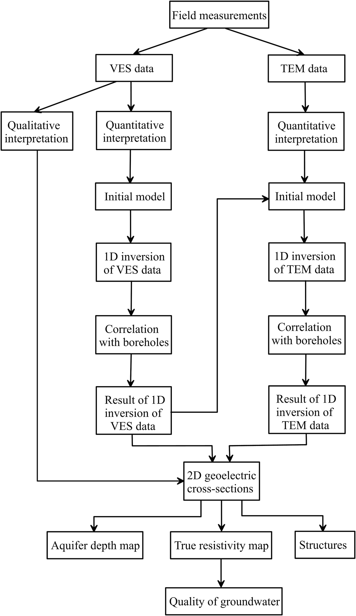
Methodological flowchart to identify the groundwater aquifer using geophysical investigations
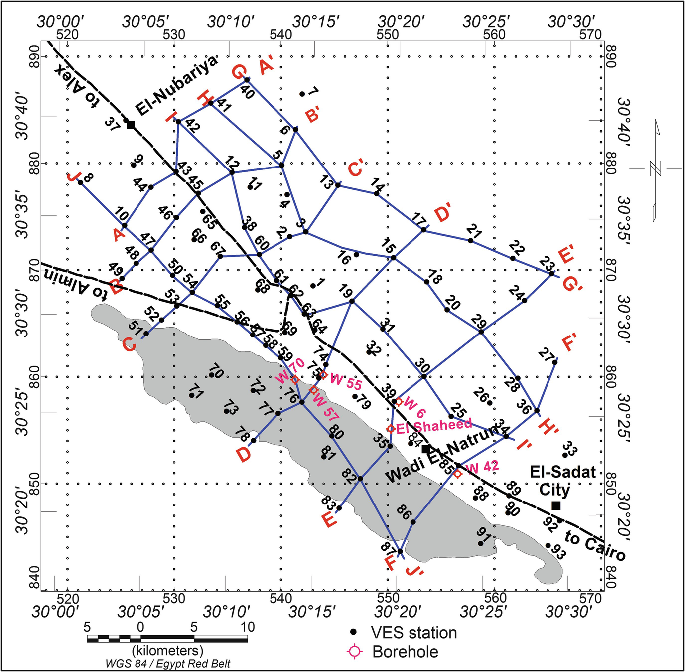
Location map of the VES stations, boreholes, and selected profiles [38]
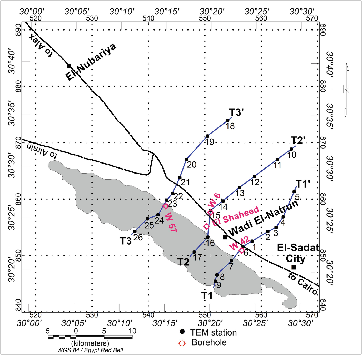
Location map for TEM stations and boreholes in the study area [38]
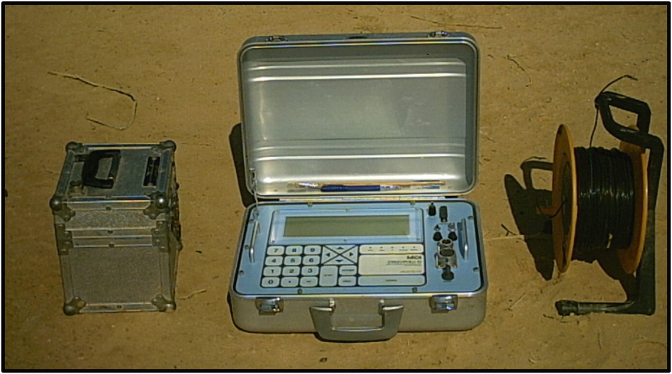
The SIROTEM MK3 TEM conductivity meter
One-dimensional resistivity inversion was carried out using the IX1D software from Interpex Ltd., which in this case solves the inversion using a ridge regression method described by Inman [61]. IX1D is a 1D direct current (DC) resistivity, induced polarization (IP), magnetotelluric (MT), and electromagnetic sounding inversion program. It supports most DC resistivity arrays, including Wenner, Schlumberger, dipole-dipole, pole-dipole, and pole-pole arrays. The RMS error is calculated by summing the squares of the difference in the log of the apparent resistivities. This result is divided by the number of data points, and the square root is taken. The antilog of this result is taken, and 1.0 is subtracted from it. Then it is multiplied by 100 to convert to percent. This method of calculating the error is used because of the large dynamic range that can be present in these data. This ensures that high apparent resistivity values do not dominate the calculated error, leaving large errors in the low apparent resistivity values [62].
8.3 Interpretation of VES Data
At each VES station, the calculated apparent resistivities are plotted against AB/2 – spacing on bi-logarithmic paper to construct the field curve for each station. The field curves were interpreted both qualitatively and quantitatively. The qualitative interpretation of the sounding curves involves the classification for the type of these curves and their aerial distribution in these areas. So, the qualitative interpretation can give an idea about the subsurface layers and their aerial distribution which will help during the quantitative interpretation.
8.3.1 Qualitative Interpretation
Qualitative interpretation of the electrical resistivity data is used to give a general view of the lateral and vertical variations of the electrical properties and to shed some light on the geological and hydrogeological conditions of the area under investigation. For the general shape of sounding curves, it has to mention that the beginning of the field curves that represent the small AB/2 values reflects the surface or near-surface variations, which is, in many cases, rapid and may confuse the main objective of this interpretation. Therefore, the resistivity behavior at large AB/2 values of the field curves is the prime importance in judging the homogeneity or inhomogeneity of the subsurface layers.
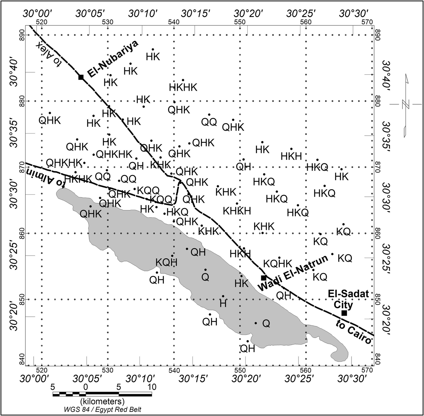
Distribution of the VES curve types in the study area [38]
Iso-apparent resistivity contour maps are also constructed for different electrode spacing to illustrate the resistivity distribution at successive levels penetrated by the artificial electric current. Each map is prepared for a given electrode separation AB/2, to illustrate the geological conditions prevailing within a horizon approximately parallel to the ground surface. Iso-apparent resistivity contour maps can outline fault zones characterized by anomalies of considerable aerial extension along a given direction and having maximum horizontal electric resistivity gradient. These maps also reveal the zones of relatively low electric resistivity values, which may indicate areas of groundwater accumulations.
- 1.
Apparent resistivity contour map of the surface layer shows variable resistivity values due to lithology heterogeneities and dryness and wetness conditions of the silt, sand, and gravel that cover the surface of the study area.
- 2.
The conspicuous lateral variations of the iso-apparent resistivities indicate comparable lateral changes in the encountered types of rocks.
- 3.
The comparison between the five iso-apparent resistivity contour maps reveals that the resistivity values generally begin with high values for the smaller depth of penetration and then decrease gradually by increasing the penetration depth.
- 4.
The study of the iso-apparent resistivity contour maps shows that the eastern region is characterized by high values and may be represented by sand and gravels. Besides, it could be deduced that the areas located in the northern and western parts (of moderated resistivity values) are saturated with shallow groundwater. Added, the low resistivity values at the area around the lakes of Wadi El-Natrun may be affected by the saltwater that comes from the lakes, or it may be represented by clay deposits.
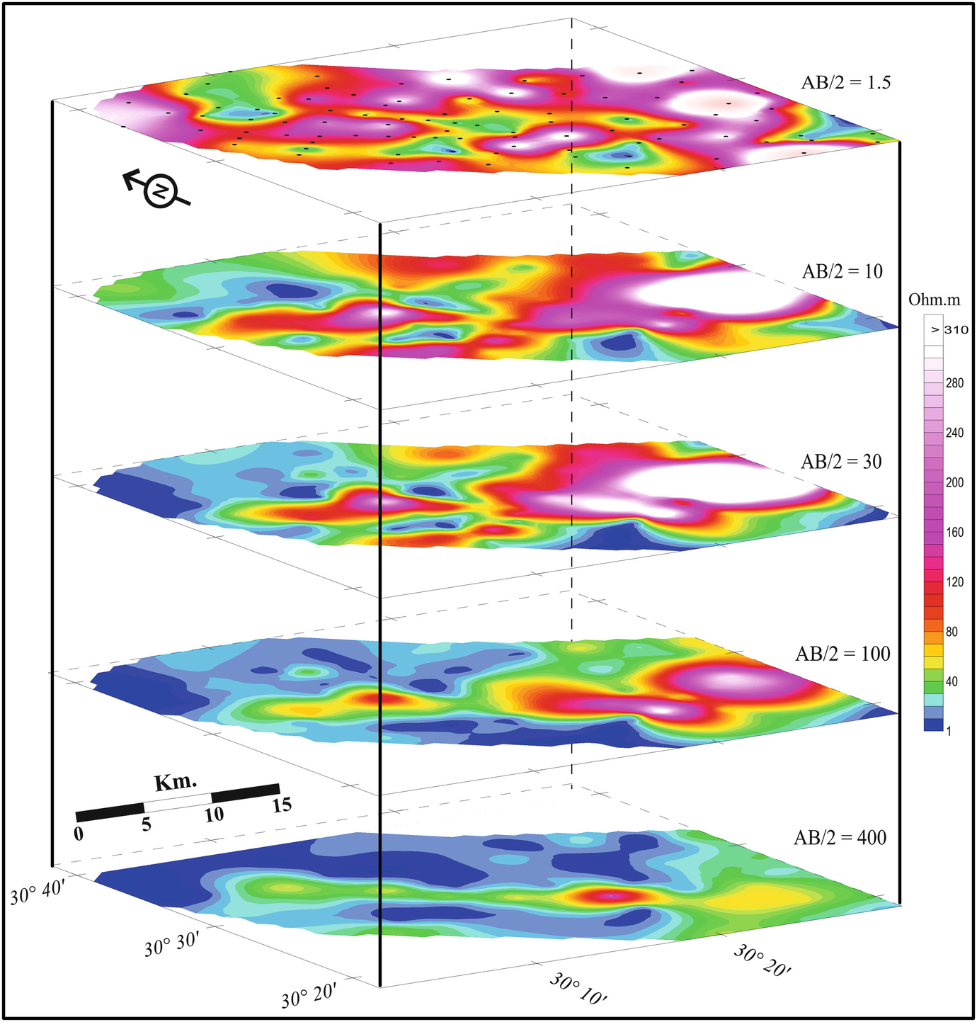
Iso-apparent resistivity maps at AB/2 = 1.5, 10, 30, 100, and 400 m [38]
8.3.2 Quantitative Interpretation
The objective of 1D modeling of an apparent resistivity curve for certain DC sounding array is to arrive, given ρ a, at the best estimate of the 1D true resistivity profile versus depth ρ z under the measurement location. This can be done either through direct transformation or through iterative, curve fitting approaches or procedures that are of a least square nature [63]. The real meaning of quantitative interpretation of the vertical sounding curves is to determine the true resistivities and thicknesses of the different formations investigated at each station along the studied sections. One-dimensional resistivity inversion was carried out in the present study using the software IX1D.
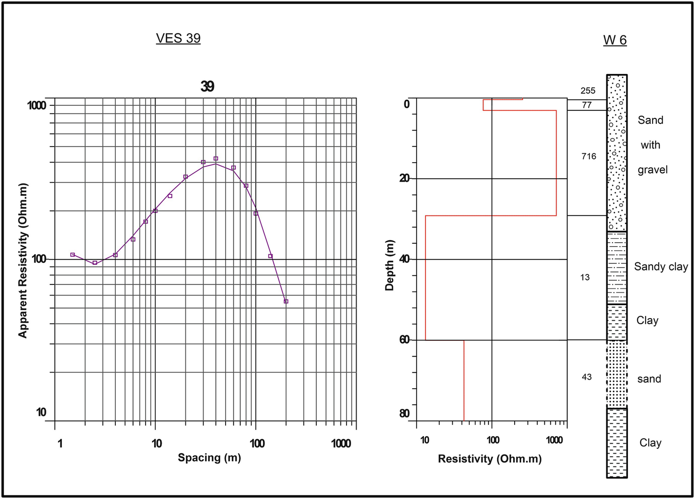
Lithology log of well 6 and its corresponding geoelectric section [38]
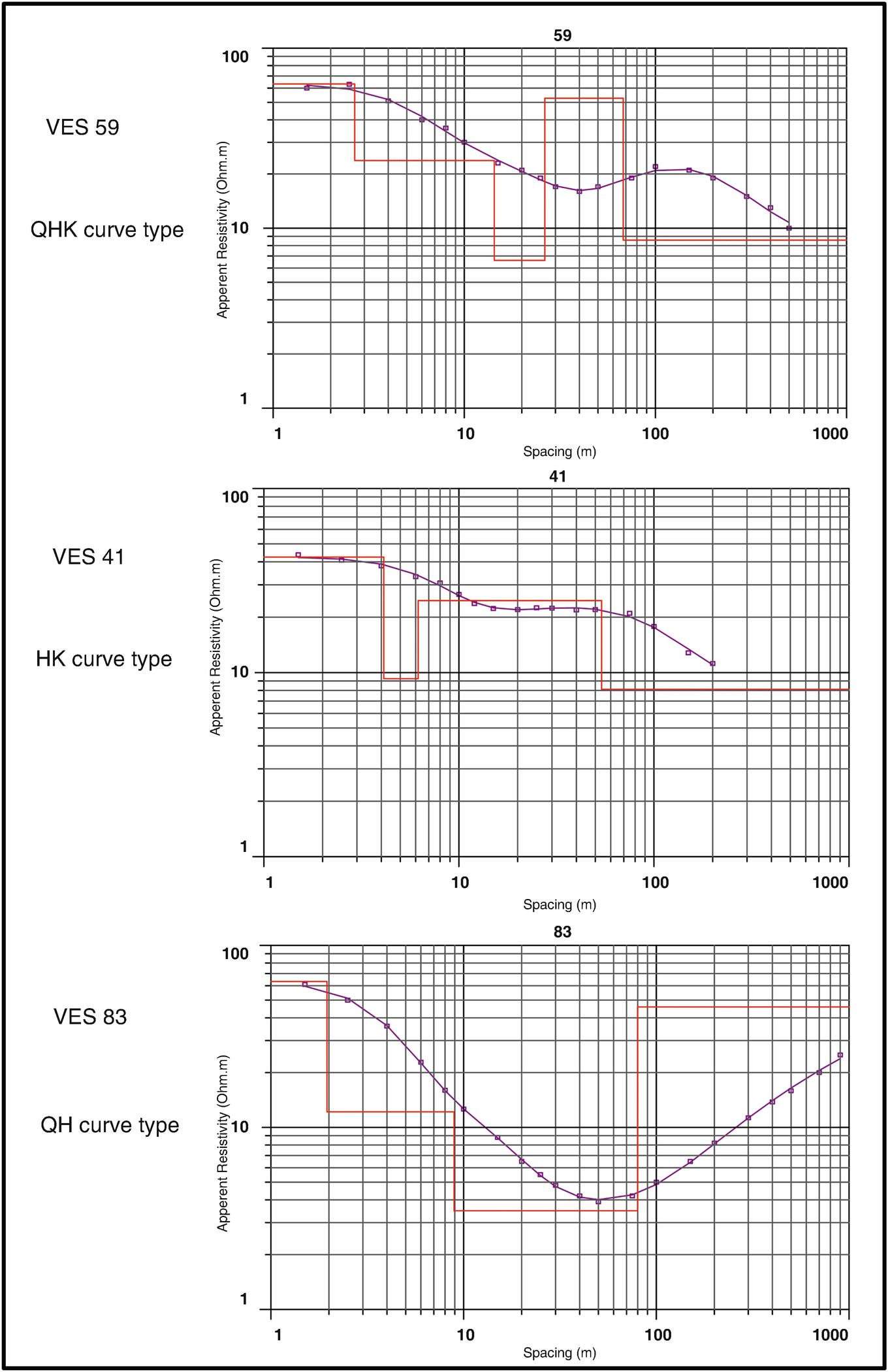
Examples of the result of the 1D inversion of VESes 41, 59, and 83
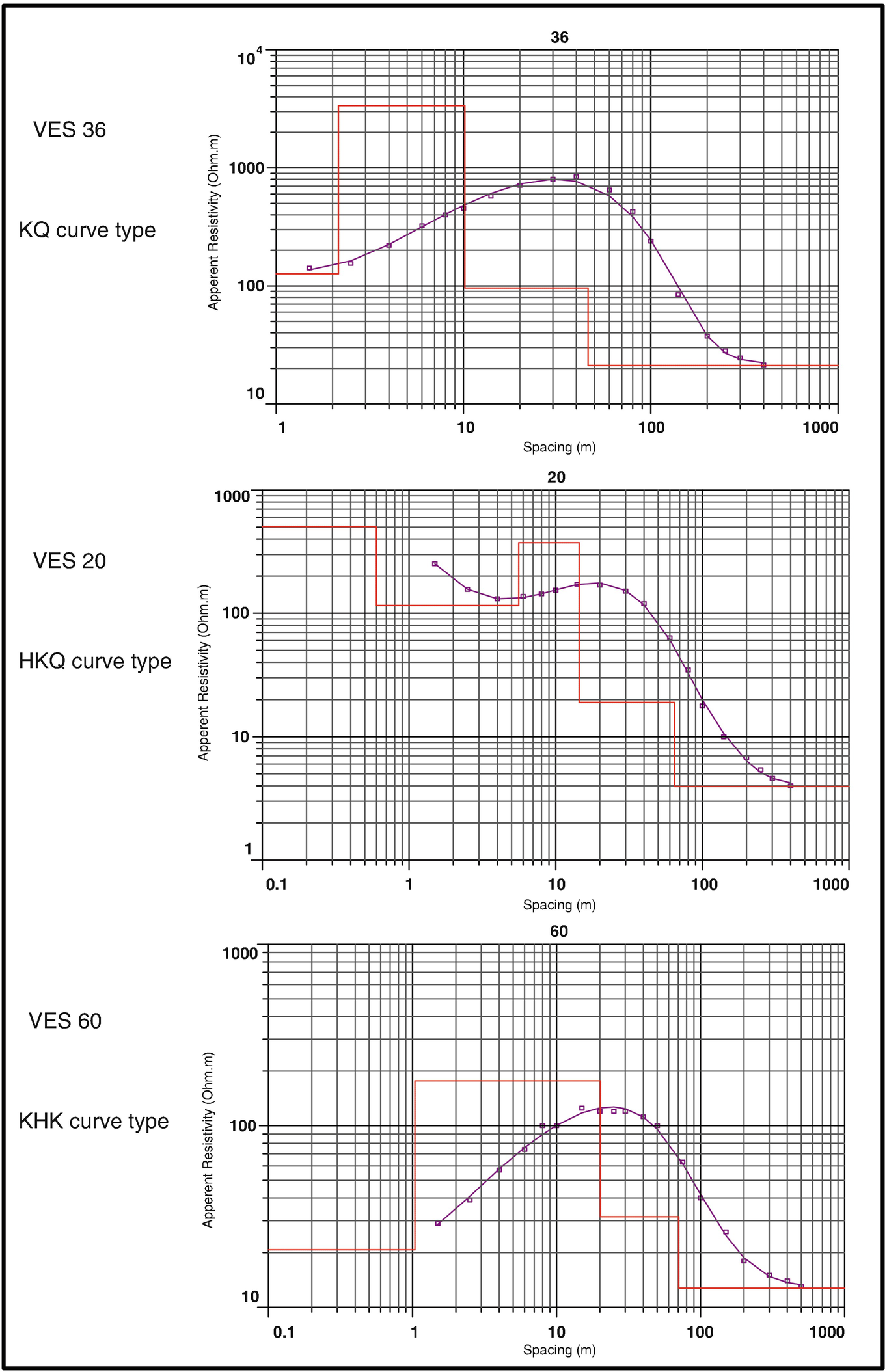
Examples of the result of the 1D inversion of VESes 20, 36, and 60
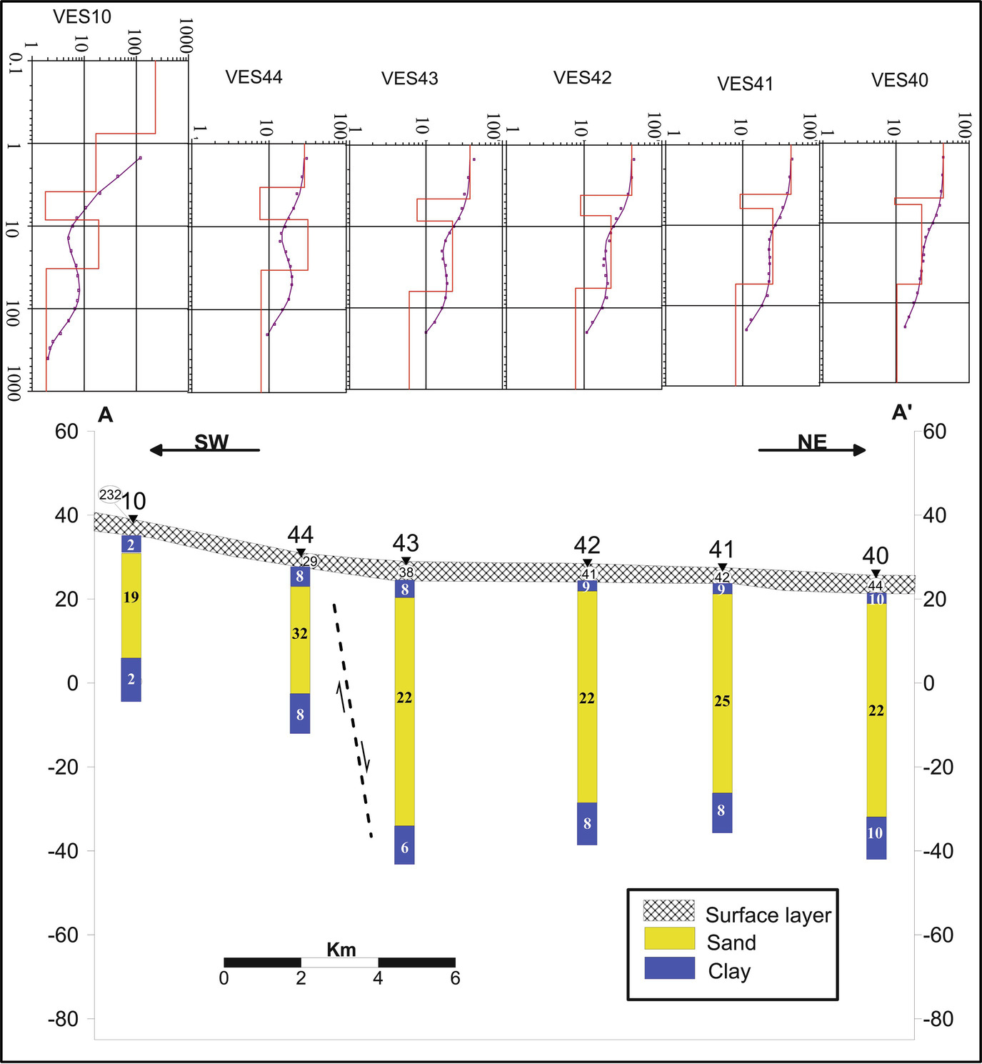
Interpreted geoelectric cross section A–A′
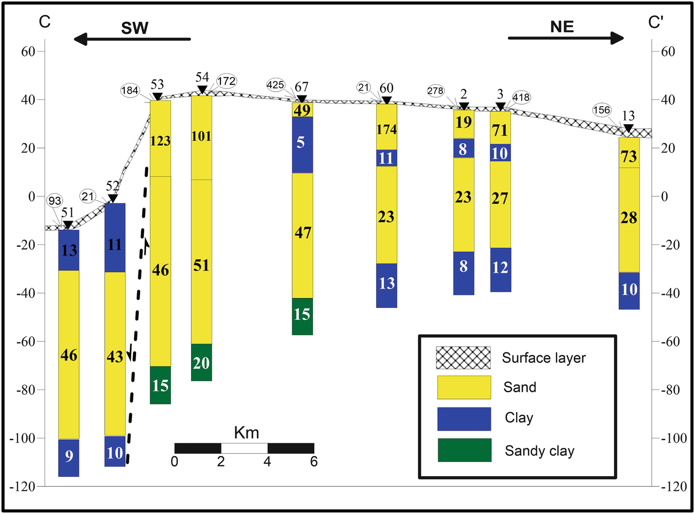
Interpreted geoelectric cross section C–C′
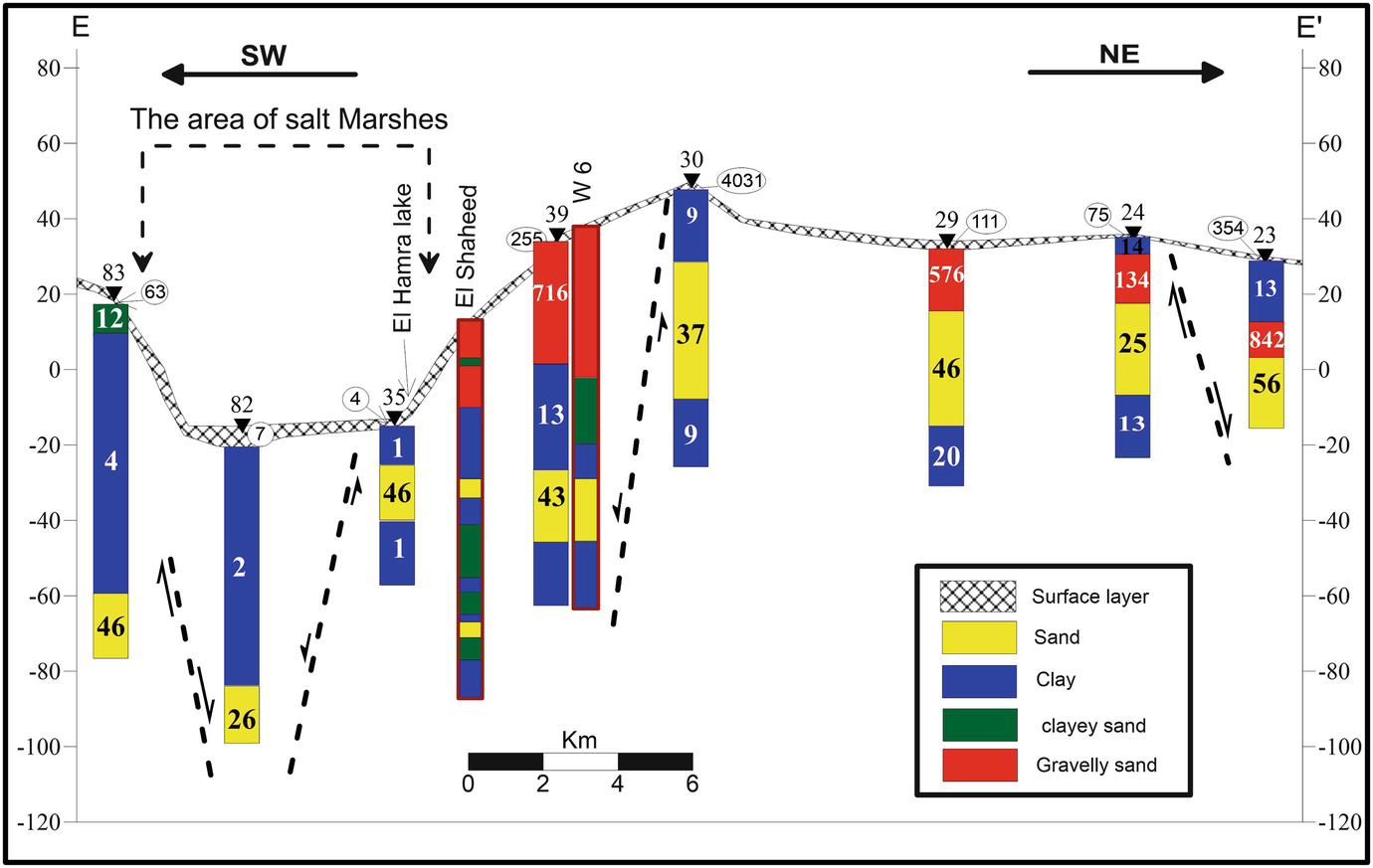
Interpreted geoelectric cross section E–E′
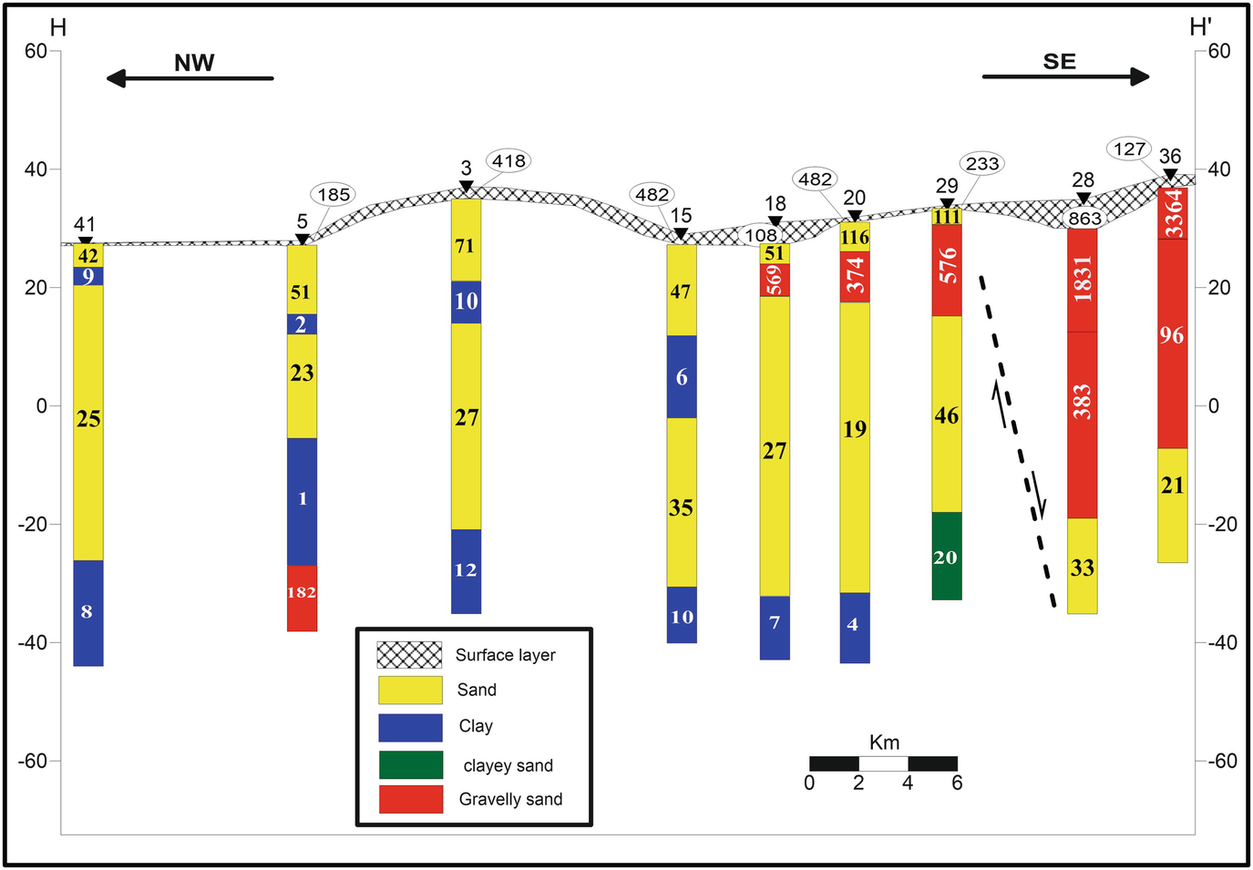
Interpreted geoelectric cross section H–H′
The first geoelectric unit is characterized by relatively very low to very high electric resistivity values ranged between 4 Ω m at VES 35 and 4,031 Ω m at VES 30. The great differences in resistivity of this layer reflect the inhomogeneity of lithology, which corresponds to sand, silt, clay, gravel, and gravelly sand. The low resistivity values are recorded in the area of salt marshes where a layer of salt covers the surface.
The second geoelectric layer shows relatively low resistivity values ranged between 2 and 15 Ω m, which corresponds to clay deposits. The thickness of this layer is ranging between 1 m at VES 40 and 44 m at VES 78. A lens of clayey sand, sand, and gravely sand that corresponds to low to high resistivity values 14–421 Ω m is found above this clay layer. This lens appears in cross sections C–C′ and D–D′.
Relatively moderate electric resistivity values ranged between 15 Ω m (VES 12) and 75 Ω m (VES 53) characterize the third geoelectric unit constituting the main aquifer in the area. The thickness of this unit is ranged between 13 m (VES 6) and 83 m (VES 53) which corresponds to sand deposits.
The fourth geoelectric unit is characterized by relatively low electric resistivity values ranged between 1 Ω m (VES 5 and VES 35) and 20 Ω m (VES 54 and VES 29) which corresponds to clay nature deposits.
Uncompleted two geoelectric layers appear only in geoelectric cross section B–B′. The first layer is recorded beneath VESes 49, 48, 47, 5, and 6. It has relatively high resistivity values ranging from 147 to 275 Ω m, which reflects gravelly sand deposits. The thickness of this layer varies from 14 m beneath VES 6 and 32 m under VES 48, whereas the second geoelectric layer is determined below VESes 49, 48, 47, and 6. This layer has relatively low resistivity values varying from 1 to 11 Ω m which leads to clay nature deposits.
8.4 Interpretation of TEM Data
The first layer is a thin layer with resistivity range between 1 Ω m at (TEMes 8, 9, and 25) and 324 Ω m at (TEM 26). The great difference in the resistivity of this layer reflects the inhomogeneity of the lithology, which corresponds to sands, silts, clay, or gravels. The thickness of this layer ranges between 0.5 and 2.8 m.
The second layer has relatively moderate to high resistivity values ranging between 57 and 265 Ω m and represents gravelly sand layer. The thickness of this layer ranges between 3.5 m at TEM 23 and 29 m at TEM 3.
The third geoelectric layer has relatively low resistivity values ranging between 1 Ω m at TEM 17 and 27 Ω m at TEM 21 and is composed of clayey sand to clay deposits. It may represent the Pleistocene aquifer. In cross section T3–T3′ (Fig. 26), this layer can be divided into three sublayers: clay, clayey sand, and clay deposits.
The fourth geoelectric layer is represented by relatively moderate resistivity values which varied from 15 to 59 Ω m. These values reflect the presence of sand and gravelly sand deposits that constitute the main Pliocene aquifer in the investigated area. The thickness varies from 9 to 57 m.
The fifth geoelectric layer has relatively low resistivity values ranging between 1 and 9 Ω m and is made up of clay. This layer is well correlated with boreholes w6, w42, and w57.
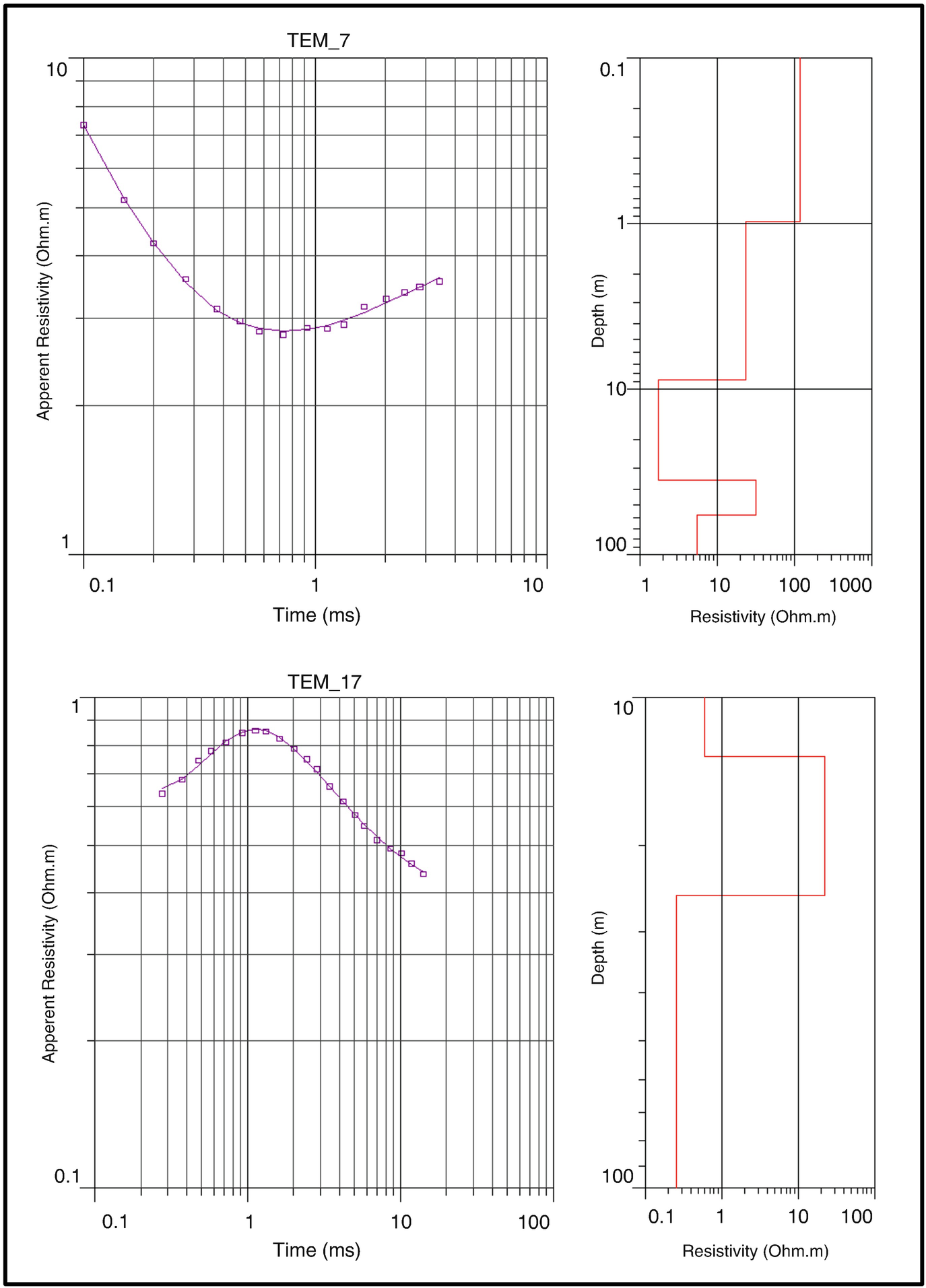
TEM sounding curves and their interpretation at stations 7 and 17
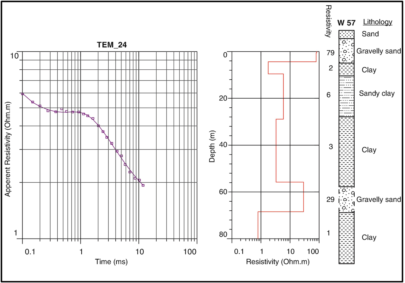
Lithology of well 57 and its corresponding geoelectric section
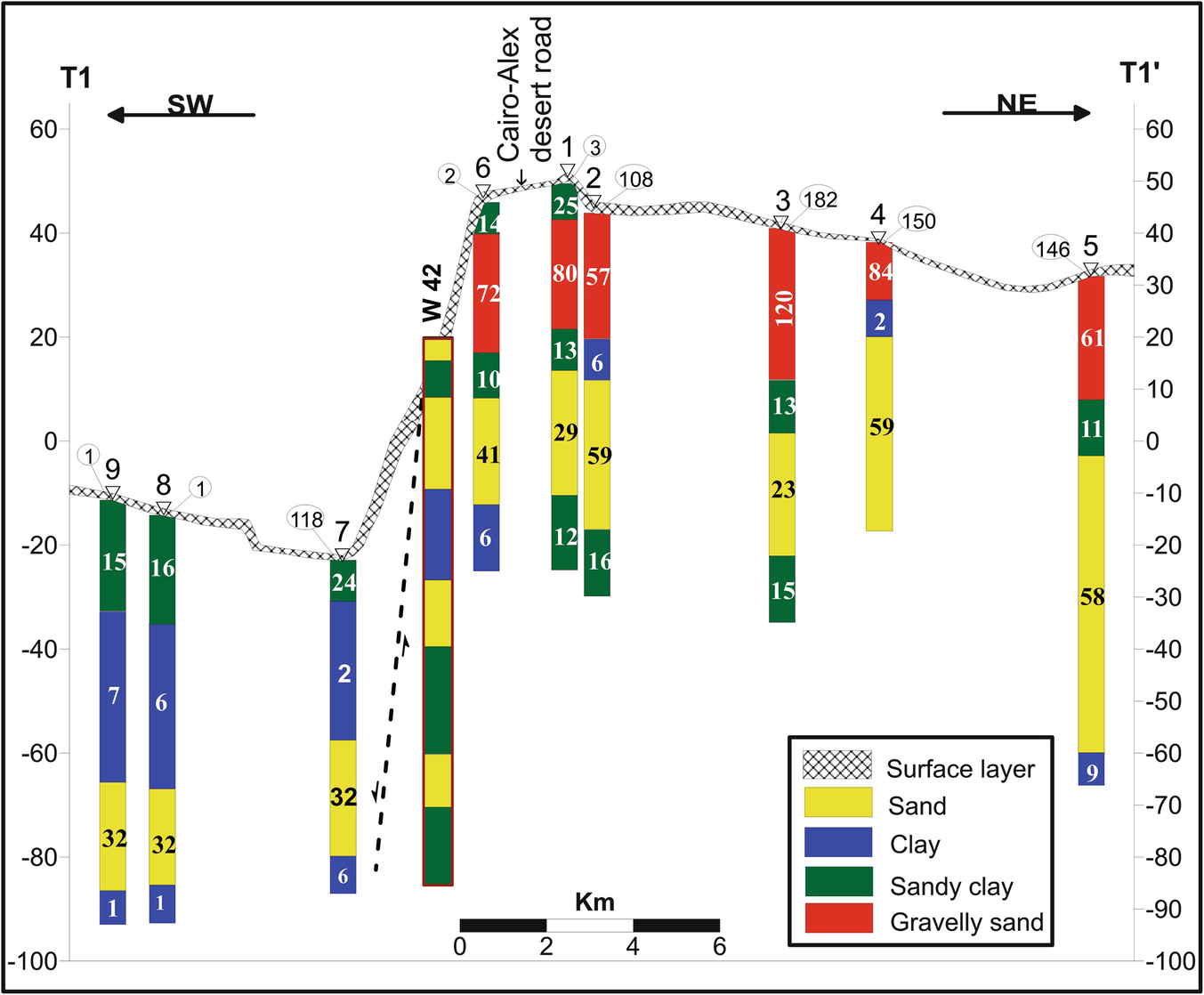
Interpreted geoelectric cross section T1–T1′
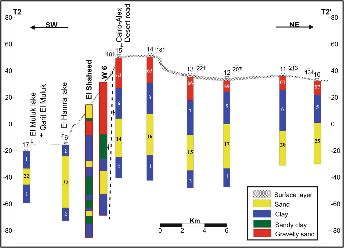
Interpreted geoelectric cross section T2–T2′
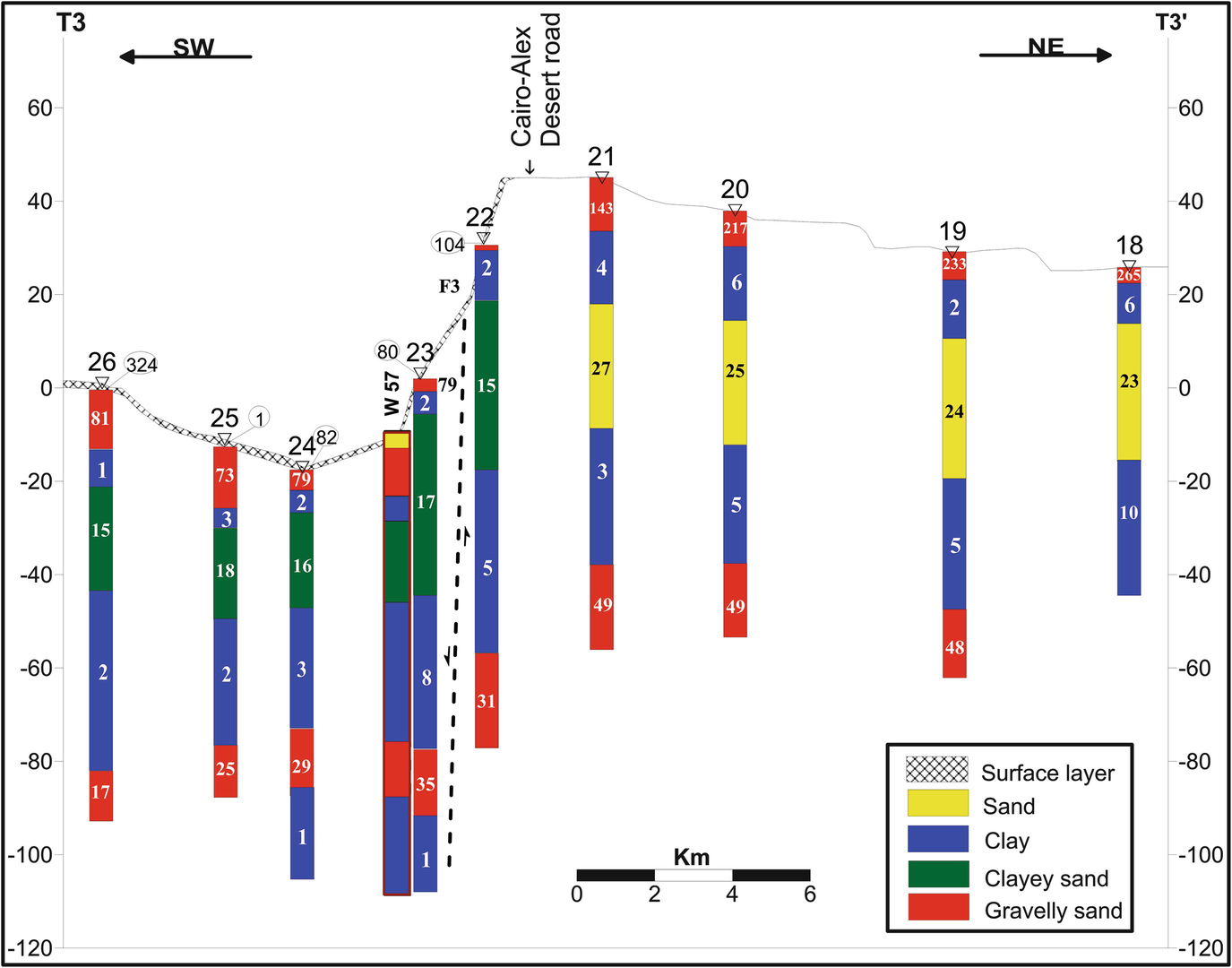
Interpreted geoelectric cross section T3–T3′
9 Results and Discussions
Depth map to the main aquifer in the study area [28]
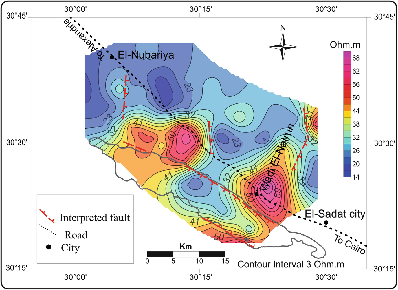
True resistivity map of the main aquifer in the study area [38]
The quality of the groundwater can be determined depending on the results of the geoelectric exploration represented by the true resistivity map (Fig. 28). A brackish groundwater can be detected at shallow depths at the northern and northeastern parts of the survey area, whereas relatively freshwater can be determined at the southern and southeastern parts around Wadi El-Natrun city at deep depths. This information should be taken into consideration during the process of drilling new boreholes. The optimum area for drilling is the northeast of Wadi El-Natrun city.
The inferred faults from the geoelectric sections were traced and collected (Fig. 28) to construct a structure map. This map shows the location and the throw of the interpreted faults in the study area. A major fault passes parallel to the northeastern edge of Wadi El-Natrun with a southwest throw. Also another fault can be detected parallel to the southwestern edge of the valley with a throw to the northeast direction. Three faults pass nearly perpendicular to Wadi El-Natrun axis with throw almost to the east which can be seen on the structure map. It is worth to mention that Wadi El-Natrun depression and its lakes are structurally controlled by set of parallel faults trending NW direction.
Saltwater of the lakes of Wadi El-Natrun causes a serious problem in the area. That is why it is worthy to have a detailed investigation to delineate the extension of the brackish water zone. Also, to the north of the study area, especially near El-Nubariya city, a shallow clay layer at depth from 1.5 to 5 m causes a trapping for the surface water; this causes a very severe problem for the crops in the area.
The results showed that TEM technique is more effective than DC resistivity technique in conductive areas where it depicts more details of subsurface layers that could not be detected by VES data, especially in the deep depths. Accordingly, it is highly recommended to apply joint inversion for the available data sets, especially VES and TEM data. Also, it is important to mention the necessity of performing 2D inversion to confirm the fault structures inferred from 1D inversion of VES and TEM data. This will be conducted in the future work of the authors.
10 Conclusions and Recommendations
The main goal of this chapter is to determine the groundwater aquifers in the West Nile Delta area. From the precise inspection of the results of the VES and TEM data interpretation, it could be concluded that the aquifer system in the area extending from Wadi El-Natrun city to El-Nubariya city along the Alexandria-Cairo desert road is divided into Pleistocene and Pliocene aquifers. The Pleistocene aquifer is the shallower aquifer and composed of gravelly to clayey sand deposits. The Pliocene aquifer is the main aquifer where it consists of sand to gravelly sand deposits. This aquifer can be detected at depth range between 6 m at the north part near El-Nubariya city to a depth of 90 m at the southern parts. The groundwater of the Pliocene aquifer can be described as a brackish groundwater at shallow depths at the northern and northeastern parts of the survey area, whereas it can be considered relatively freshwater at deep depths at the southern and southeastern parts around Wadi El-Natrun city. Based on the structural map inferred from the 2D geoelectric cross sections, it is worth to mention that Wadi El-Natrun depression is structurally controlled by a set of parallel faults trending NW.
We found that DC resistivity technique is very appropriate in determining the subsurface layers at shallow depths with a high resolution. On the other hand, TEM technique is more effective than DC resistivity technique in detecting more details of subsurface layers that could not be detected by VES method, especially in the deep depths. Accordingly, it is highly recommended to apply TEM and DC resistivity techniques together in groundwater studies.
In case of drilling new boreholes for drinking or agricultural purposes, we recommend the area northeast of Wadi El-Natrun city. Also, the saltwater of the lakes of Wadi El-Natrun causes a serious problem in the area. That is why it is worthy to have a detailed investigation to delineate the extension of the brackish water zone. We also recommend installing a covered drainage system to overcome the problem of trapping surface water near El-Nubariya city.