1 Introduction
Geoelectrical methods are increasingly popular in detecting and characterizing aquifers as the resistivity of sediments and rocks depends mainly on their water and material contents (e.g., [1–3]). One of such electrical methods is direct current resistivity (DCR) technique. In DCR method, the potential difference is measured via injecting DC into the ground with electrodes at the ground surface. The DCR method has received a great attention because of its potential applications in the field of hydrogeology and saltwater intrusion tomography [4, 5]. In the arid and semiarid region, the DCR method is popularly used for groundwater exploration and aquifer mapping (e.g., [6, 7]). This can be attributed to the rapid advancement in the development of digital modeling solutions and electronic technology of hydrogeological problems (e.g., [8]). Besides the efficiency of such method for lithological characterization, the DCR technique has led to many studies on hydrogeological parameter estimation of the aquifer (e.g., [9]). On the other hand, in the coastal areas, the DCR imaging is suitable for monitoring saltwater intrusion and groundwater contamination as this method quickly investigates a large site without needing for well drilling (e.g., [10]).
Induced polarization (IP) technique is one of the geoelectrical methods based on studying the low-frequency polarization processes taking place in porous media. Generally, the IP method extends from the classical DCR method. Basically, IP measures the earth’s capacity to store an electric charge over time. Accordingly, after the injected current is shut off, the voltage decay curve is measured; the higher the IP, the longer over time the stored charge. It is well known that IP is a considerable and useful method for mineral exploration. On the other hand, the real and imaginary parts of conductivity are measured over a range of frequencies in spectral induced polarization (SIP). The resistivity amplitude and the phase shift between the input current and measured voltage can be recasted into a complex conductivity. Recently, the SIP method has shown its potential to predict the petrophysical parameters in saturated conditions at the field and laboratory scales (e.g., [11, 12]). Usually, DCR method is the preferred, but the resistivity data interpretation suffers from a major flaw: the inability to discriminate between surface and bulk conductivity. This causes unrealistic interpretation in hydrogeophysics. Such main problem can be resolved by using SIP method (e.g., [11, 13, 14]).
In Egypt, the River Nile is the lifeline, where the main water source is surface water from the River. With increasing populations, urbanizations and land reclamation projects in Egypt, the surface water from the River Nile is not sufficient. The groundwater is the second important water resources. Furthermore, the saltwater has intruded from the northern and eastern parts of Egypt along the Mediterranean Sea and Suez Canal, respectively. Additionally, the overpumping of groundwater at the northern parts causes vertical upwelling of saltwater from deeper parts causing degradation to groundwater quality. It can also be noticed that a large part of agricultural areas in the northern parts has been, consequently, affected by saltwater intrusion. Accordingly, the groundwater assessment and management have become extremely important.
This chapter attempts to guide the reader to some of the important sources of information on the use of DCR and IP methods for groundwater assessment. In the first section of this chapter, fundamental of DCR and IP methods will be explained. The linkage between the data of geoelectrical and hydraulic characteristics at the field and laboratory scales will be discussed. The geoelectrical data inversion techniques will be briefly covered in the second section of this chapter. Practically, three cases studied from Nile Delta are presented in the third part. Here, a saltwater intrusion and groundwater resource characterization, i.e., hydrogeophysical characterization, in coastal and semiarid areas, respectively, are reported.
2 DC/IP Resistivity Methods
2.1 Fundamentals
Resistivity values of common earth’s materials and chemicals [16]
Materials | Resistivity (Ω m) |
|---|---|
Igneous and metamorphic rocks | |
Granite | 5 × 10³–106 |
Basalt | 103–106 |
Marble | 102–2.5 × 10⁸ |
Quartzite | 102–2 × 10⁸ |
Sedimentary rocks | |
Sandstone | 8–4 × 10³ |
Shale | 20–2 × 10³ |
Limestone | 50–4 × 10² |
Soils and water | |
Clay | 1–100 |
Alluvium | 10–800 |
Groundwater (fresh) | 10–100 |
Saltwater | <1 |

ρ w is the water resistivity, ρ is the formation resistivity, a is an empirical constancy (typically 1 for unconsolidated sediments), m is an empirical constant (typically 2 for unconsolidated sediments), φ is the effective porosity, and F is the formation factor related to the volume and tortuosity of the pore space.
2.2 Physical Base
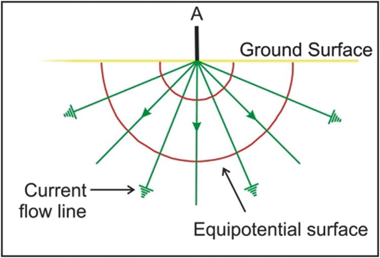
Simplified current flow lines and equipotential surfaces arising from a single current source
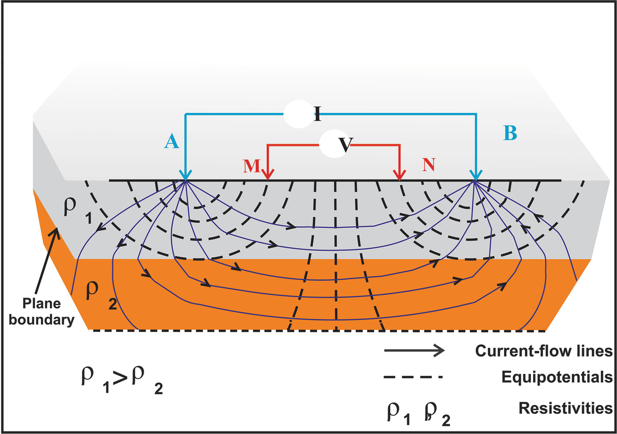
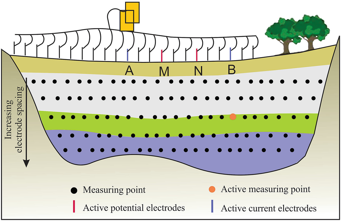
Resistivity measurement principles with a four-electrode configuration


where K is the geometrical factor having the dimension of length (m), which depends on the arrangement of the four electrodes.
The IP method is considered as an extension to the well-known geoelectric technique. It is usually assumed that IP and DCR measurements have been measured simultaneously. The IP method depends mainly on a small amount of electric charge storage when a current is passed through the rock, to be released and measured when the current is switched off. Generally speaking, the IP measurements became more established in the last 20 years.


In the spectral induced polarization (SIP) method, the resistivity/conductivity magnitude and phase shift are measured over a wide range of frequencies (0.625 Hz to 10 kHz).


where ω is the angular frequency and σ′ and σ″ are the real and imaginary parts of the electrical conductivity, respectively.
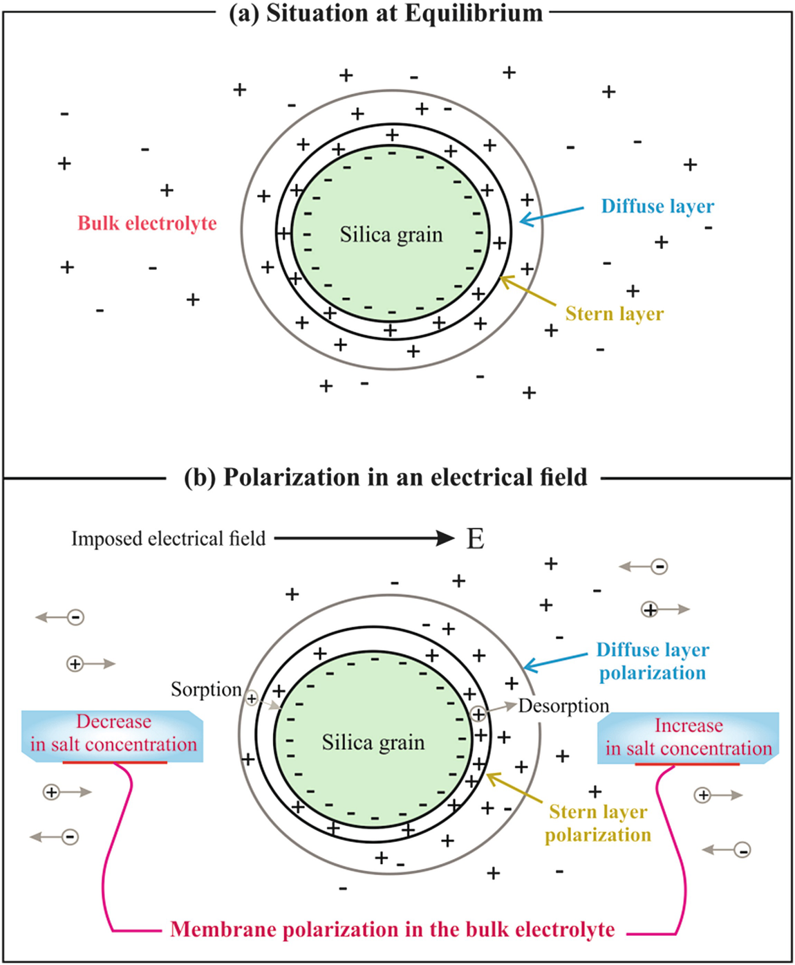
A single grain polarization. (a) Electrical double layer (Stern plus diffuse layers) at equilibrium. (b) Polarization mechanisms of the grain under an electrical field E (modified after [20]).
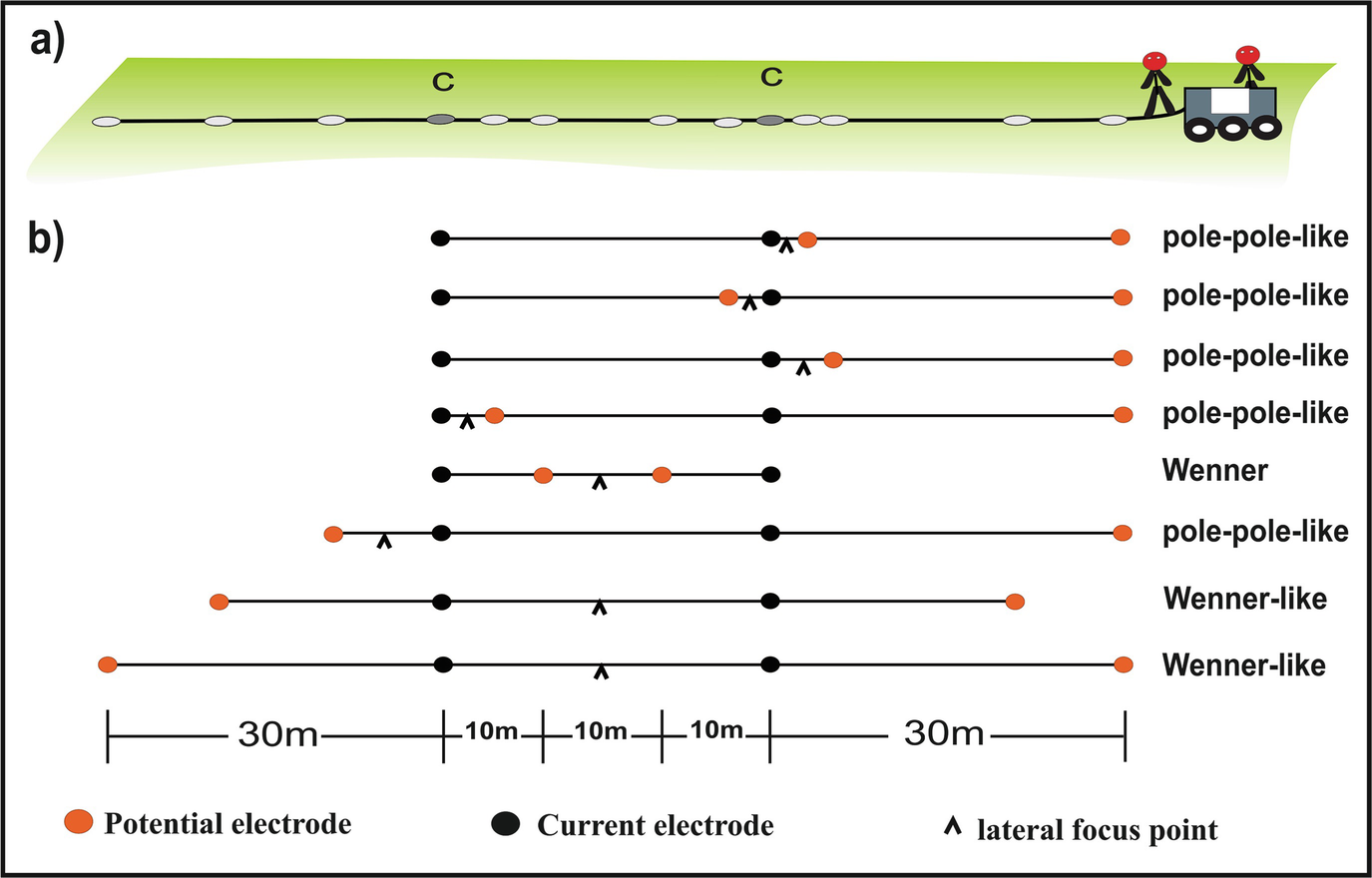
2.3 Electrode Arrays and Field Techniques
- 1.
The structure types to be mapped, the resistivity instrument sensitivity, the noise level, the signal strength, and the data coverage
- 2.
The array sensitivity to vertical and horizontal changes in the subsurface resistivity (e.g., [27])
- 3.
The depth of investigation (DOI) [28]
- 4.
The array resolution for horizontal and dipping layers and sensitivity to surface heterogeneous [29]
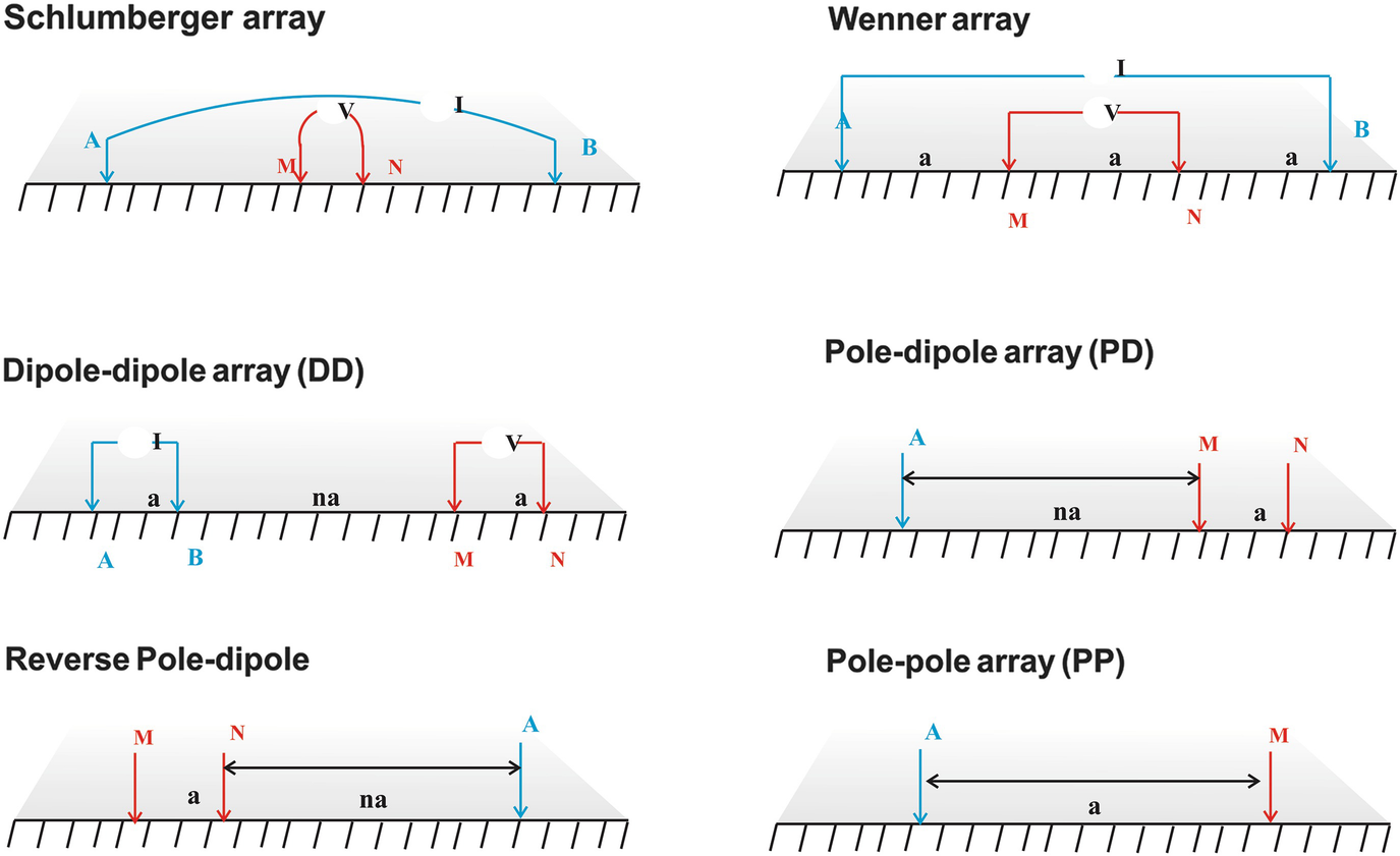
Some of the most commonly used electrode arrays. The letters A and B designate the current electrodes, and the letters M and N denote the potential electrodes
A schematic model of the CES technique and data density using Wenner array
A schematic model of the PACES system (a) showing the pulled electrodes by a small caterpillar using eight-electrode configurations (b)
2.4 Hydraulic Conductivity Prediction


The correlation of K with ρ′ is directly proportional on a large scale for sandy-clayey aquifer [11]. On a local scale, sometimes, such correlation is inversely proportional [32].


where σ″ in mS/m and Spor is in μm−1.

where σ″ is given in μS/m. m and n are adjustable parameters with m = (2.0 ± 0.3) 10–4; n = 1.1 ± 0.2, and K is in m/s.

where a and b are formation-specific parameters.

The four empirical parameters a, b, c, and d are determined by a multivariate regression analysis.

2.5 Geoelectrical Data Inversion
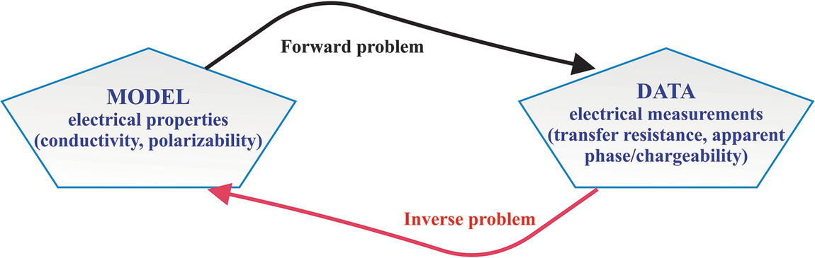
DCR interpretation process in the form of forward and inverse problems
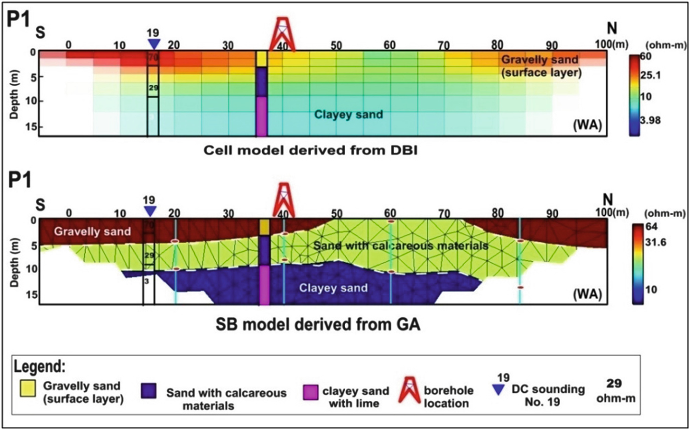
2D ERTs obtained from Wenner alpha (WA) data using (top) DBI method and (bottom) nonconventional inversion method produced by GA and structure-based (SB) model. Note that (bottom) all model nodes (pink dots over white circle) along the control points (turquoise color) defining the layer interfaces were derived from the borehole information and the preliminary DBI results
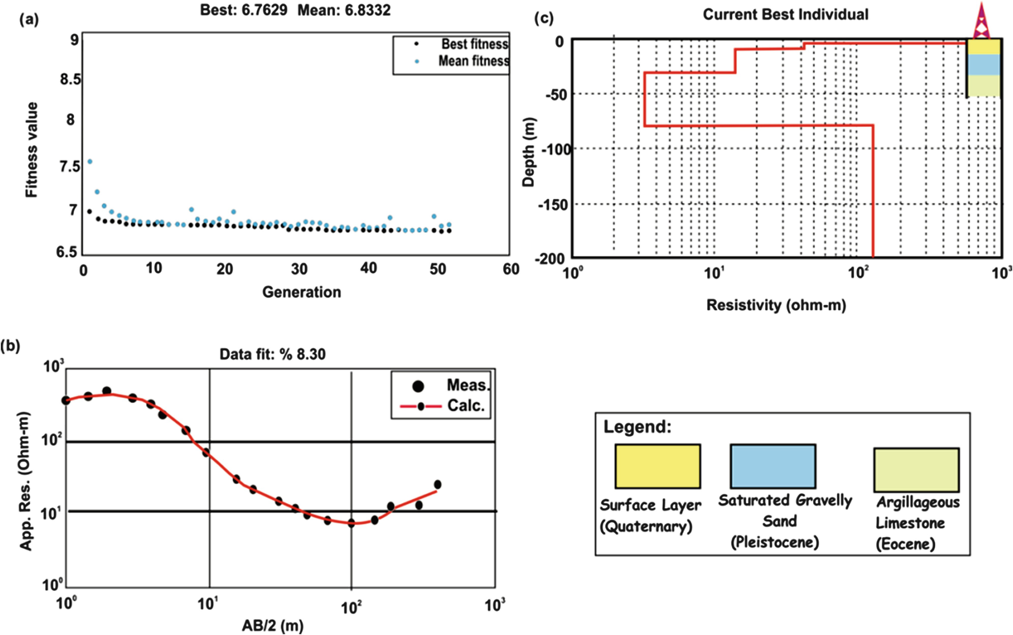
The interpreted resistivity layers constrained with the geological data using a genetic algorithm (GA); (a) variations of mean and best misfit versus generation; (b) a comparison between the measured and calculated data at the best misfit value; (c) a comparison between the model response and borehole information
3 Applications to the Nile Delta

3D visualization resistivity model represents the resistivity distributions at the northern part of the East Nile Delta, Egypt [4]
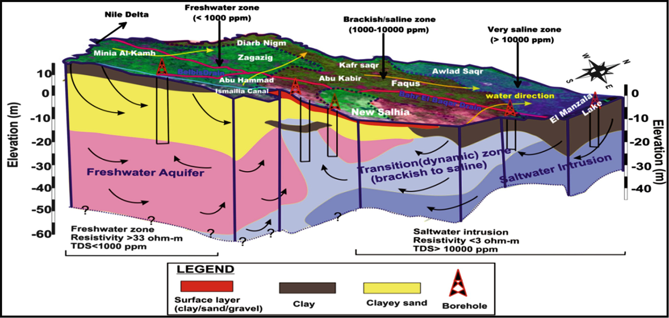
3D schematic model shows the freshwater/saltwater conditions at a coastal area, East Nile Delta, Egypt [4]
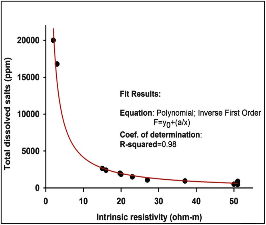
Correlation between true resistivity derived from DCR sounding inversion and TDS of some collected water samples at the northern coastal part of East Nile Delta [4]
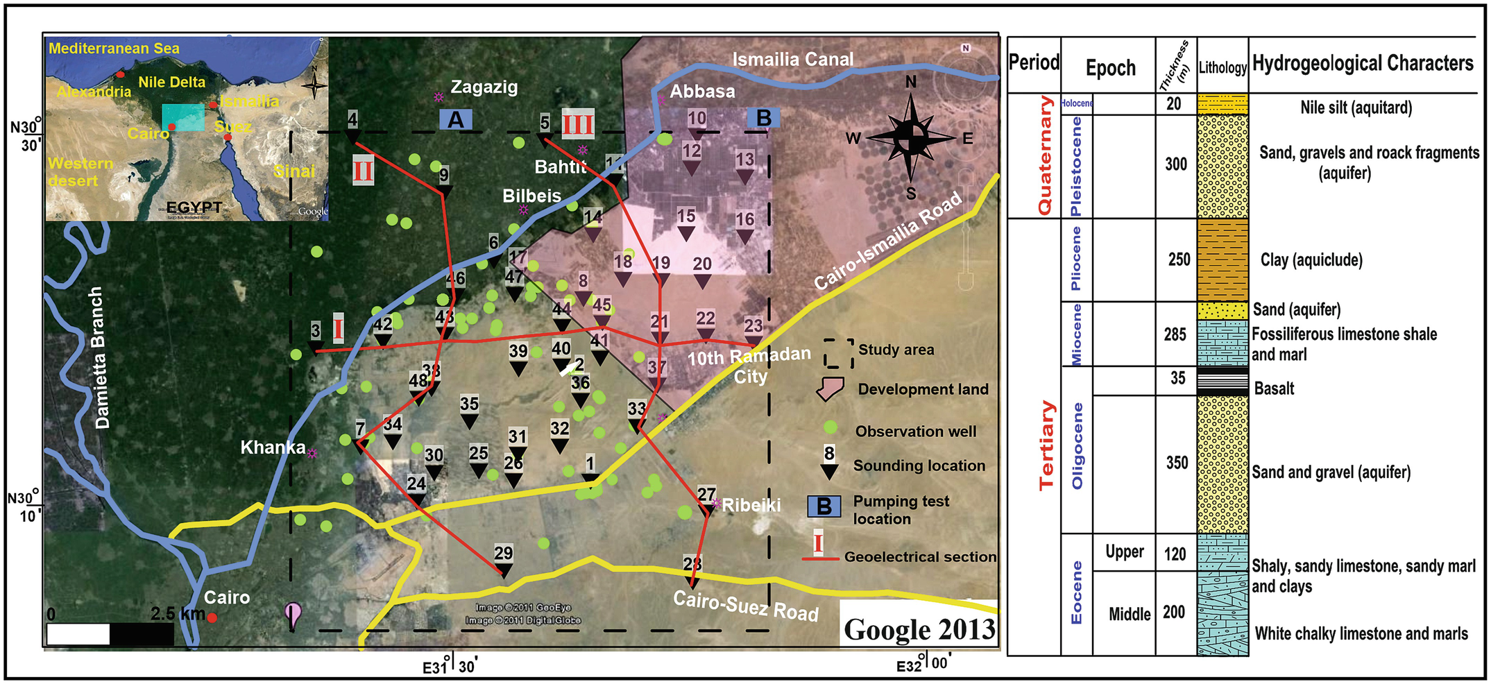
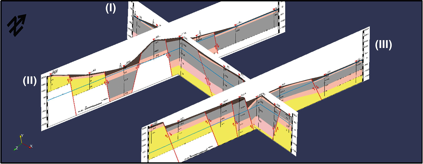
Location map of the East Nile Delta showing the DCR soundings, geoelectrical cross section, and observed boreholes (left panel). Compiles stratigraphic section (right panel) of the East Nile Delta
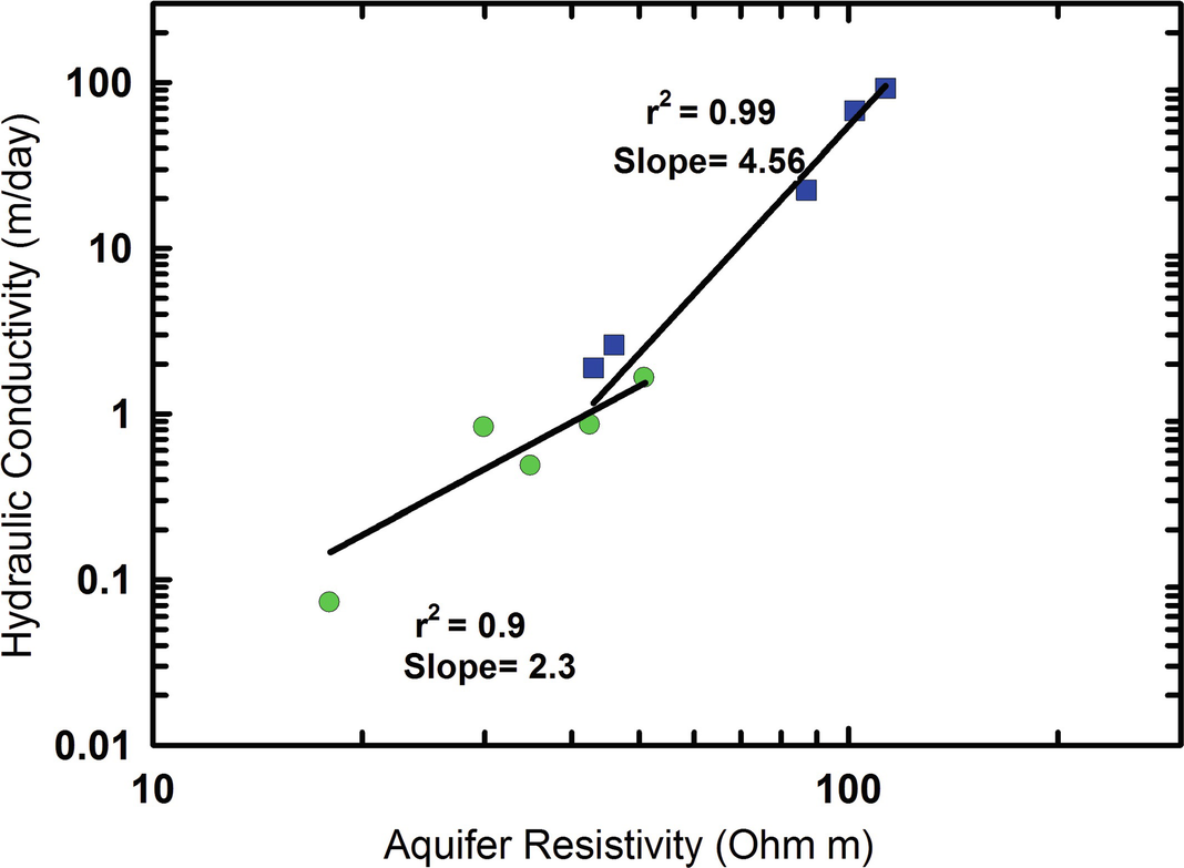
The aquifer resistivity vs. the hydraulic conductivity (K) of ten DCR soundings and observed boreholes. Blue solid squares indicate Quaternary aquifer, while the Tertiary aquifer is represented by green solid circles [2]
4 Conclusions and Recommendations
The chapter shows that the application of DCR method with available boreholes, an integrative approach, is valuable in hydrogeological conditions assessment in East Nile Delta, Egypt. Based on the present studies from East Nile Delta, the results proved (1) the efficiency of the DCR method for hydrogeological evaluation in costal semiarid areas and (2) the validity of the DCR method to predict the TDS and K using the empirical relationships for this area. Furthermore, the joint use of the conventional and nonconventional inversion techniques is recommended for hydrogeological evaluation in East Nile Delta. In the ongoing research, the computational speed of GA requires to be improved applying parallel computation. Further research including pumping tests is required to verify the prediction of hydraulic conductivity using the geoelectrical empirical relationships in East Nile Delta. Additionally the derived salinity equation modification is desirable considering the clay content ratio and grain size analysis. Therefore, it is worthwhile to mention that the DCR method has a great importance for hydrogeological assessment to the decision-makers.