Groundwater Potential in the New Valley South West of the Nile Delta in Egypt

Abstract

Egypt is continuously facing a decrease in water share per capita due to a decline in available water resources.

The objective of the present study is to evaluate and manage the groundwater resources of the Nubian Sandstone Aquifer System (NSAS) in the New Valley area. It is located in the middle part of Egypt’s Western Desert. It lies between latitudes of 24°–28° N and longitudes of 27°–31.5° E. It covers an area of 440 km long by 460 km wide where the total area is about (202,400 km²). A detailed review of the Nubian Sandstone Aquifer in the western desert is also introduced.

A finite difference model using “Visual MODFLOW” was applied on the Nubian Sandstone Aquifer of Dakhla Basin. It was adapted to simulate groundwater flow in such aquifer. The simulation was calibrated with available groundwater head data from CEDARE Report (2002). An optimum solution is established for the safe groundwater mining in the study area.

The scenario applications could allow for an increase in reclamation at Dakhla Oasis by 15%, with the condition of safe drawdown values less than 60 m for the period of 100 years.

The study provides the benefits of applying the modeling techniques. Numerous valuable inputs for the national development plan in Egypt are presented. The study found that it is important to seek an alternative water resource to compensate for the groundwater depletion.

1 Introduction

Groundwater is one of the most important resources of water in Egypt, ranking second after the River Nile. Although in terms of quantity the contribution of groundwater to the total water supply in Egypt is very moderate. Groundwater is the only available source of water for people living in the desert area. In terms of quality, groundwater, unless contaminated, is generally of better quality than surface water. The quality of groundwater depends on two main factors, namely the origin of the water and the type of rocks bearing it. Groundwater is obtained in many areas from fissures, and joints of the igneous and metamorphic rocks. It may be found in layers of weathered basement rocks. It can also be extracted from alluvial deposits and aquifers in coastal areas.

Demand for water has increased during the last decade particularly due to the declining availability of freshwater. This has expanded the development of searching and extracting groundwater resources. An evaluation of the renewable groundwater resources is essential for any Integrated Water Resource Management (IWRM) plans that are sustainable. In this study, the evaluation of the renewable groundwater resources in Egypt from water quality and quantity perspective is discussed.

2 Groundwater System in Egypt

The aquifers systems in Egypt are distributed over the country and the hydrogeological framework of Egypt. It can be characterized into eight hydrogeological units as shown in Fig. 1 [3, 4]. These units are:

1.
Nile Valley and Delta aquifers,
2.
Coastal aquifers,
3.
Moghra aquifer,
4.
Aquiclude rocks,
5.
Carbonate rocks complex aquifers,
6.
Nubian Sandstone Aquifer,
7.
Fissured basement complex aquifers, and
8.
Tertiary aquifers
Fig. 1
The aquifer systems of Egypt. Modified after RIGW [1, 2]

They differ in general characteristics, including extension, hydraulic conductivity, transmissivity, storage, and recharge.

The above-mentioned aquifers are classified into two groups based on the water-bearing rocks as given in Table 1:

1.
Granular water-bearing rocks and
2.
Fissured and karstified water-bearing rocks

Table 1

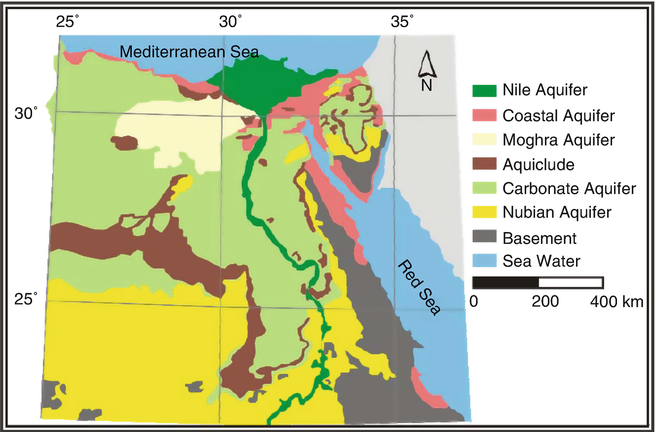
The main hydrogeological units in Egypt [3]

Lithology rock type	Unit	Recharge		Distribution	Productivity
Lithology rock type	Unit	Surface	Sub-surface	Distribution	Productivity
Granular material	Nile Valley and Delta	Continues	Continues	Extensive	High
	Coastal aquifer	Occasional	Limited	Local	High
	Nubian Sandstone	None	Limited	Extensive	High

The Nubian Sandstone Aquifer is selected for further study in this respect since it is considered the main groundwater resource in the New Valley in the Western Desert of Egypt.

3 Regional Nubian Sandstone Aquifer System

The Nubian Sandstone Aquifer system is a regional system. It extends into Libya, Sudan, and Chad. It is a nonrenewable aquifer system [5]. The Nubian aquifer system (Fig. 2), one of the largest groundwater systems of the Sahara, is formed by two major basins: the Kufra Basin in Libya, north-eastern Chad and northwestern Sudan, and the Dakhla Basin of Egypt. In addition, the aquifer area includes the southernmost strip of the northwestern Basin of Egypt and the Sudan Platform 7, Brinkman et al. [8].

../images/437178_1_En_62_Chapter/437178_1_En_62_Fig2_HTML.png — Fig. 2
Regional hydrogeological overview of the Nubian Sandstone Aquifer System. Compiled from: CEDARE [6] and Bakhbakhi [7]

The total area is about two million square kilometers. The Nubian Sandstone Aquifer in Egypt is assigned to the Paleozoic–Mesozoic. It occupies a large area in the Western Desert and parts of the Eastern Desert and Sinai.

“In spite of its vast area, it is considered as a broadly closed system, as it has natural boundaries to the east and southeast formed by the mountain ranges of the Nubian Shield and is bounded to the south and west by the mountainous outcrops of Kordofan Block, Ennedi, and Tibesti. To the southwestern part of the basin, the aquifer is bounded by the groundwater divide located between Ennedi and Tibesti Mountains. The natural northern boundary of the Nubian Sandstone Aquifer System is set to the so-called Saline-Freshwater Interface, whose location is considered spatially stable, although slight movement is believable,” Sefelnasr [9, 10].

“Groundwater can be found at very shallow depths, where the water-bearing formation (Horizon) is exposed or at very large depths (up to 1,500 m),” where the aquifer is semi-confined. “The deepest water-bearing horizons are generally encountered in the North,” as in the Siwa Oasis, while the shallowest are encountered in the southern portion of Kharga and the East Oweinat area. The aquifer transmissivity is generally medium to low, varying from 1,000 to 4,000 m²/day, Sefelnasr [10].

CEDARE/IFAD [6] in a program for the development of a regional strategy for the utilization of the Nubian Sandstone Aquifer System has estimated the fresh groundwater volume within the system at 372,950 km³.

“Groundwater quality is generally good in the major part, except near the coastal regions and Sinai,” RIGW [11] and Sefelnasr [10].

The following section is discussing in more detail the most recent study for the groundwater potential in the New Valley area of Egypt [12]. The objective of this study is to evaluate and manage the use of the valuable groundwater resources of the Nubian Sandstone Aquifer System (NSAS) in the study area. It is located in the middle part of Egypt’s Western Desert. It lies between latitudes of 24°–28° N and longitudes of 27°–31.5° E. It covers an area of about 440 km long by 460 km wide (about an area of 202,400 km²).

4 Conceptual Model

The hydrogeological groundwater flow modeling is based on a valuable tool to better understanding groundwater flow in aquifers and to better managing groundwater resources. Numerical models are one of the few tools available that can consider a complex array of aquifer variables (hydraulic properties, recharge, pumping, rivers, structure, and heterogeneity) and allow these variables to interact with themselves. Exploring these interactions with a model can be used to make predictions important for managing groundwater resources, such as predicting how water levels might respond to increased pumping or drought.

The model study area of “Dakhla Basin includes Farafra, Dakhla and Kharga Oases.” The Dakhla basin includes the upper Post Nubian Aquifer, separated from the Nubian by an aquitard. However, the model study includes the main deeper aquifer since the upper post-Nubian aquifer is almost declining and that it is not feasible to include it in the study. For this reason, the upper aquifer will be considered inactive in this model study. The Nubian aquifer in this respect still contains a huge groundwater storage that can help in the development of the New Valley region, provided that good water management plan is required since this Nubian system is not well recharged and should be treated as groundwater mining aquifer.

Based on the hydrogeological map of Egypt (Fig. 3a) and the schematic cross sections shown in (Fig. 3b, c), they were schematized as the series of layers. The upper layers are considered as zone 1and the Nubian Sandstone Aquifer is considered as zone 2, as follows:

The oldest and most extended aquifer comprises the Paleozoic and Mesozoic continental deposits (zone 2). It is older than the Upper Cinemania (zone 1). A large part of the lower aquifer is exposed south of the 26° N parallel and is in unconfined condition.
More recent groundwater reservoir includes the Tertiary Carbonate rocks in western Desert of Egypt. However, this aquifer is heavily depleted, and most of the wells are becoming dry which forced the natives in the area abandon those wells and replace them with deeper wells drilled in the deep Nubian aquifer.
The two zones are separated by an impermeable shale layer (aquitard or confining bed) above which the Upper Cretaceous deposit is located.
According to the aforementioned discussion, it is only feasible to develop the lower deep Nubian aquifer. In this situation, the upper aquifer in zone 1 will be discarded because most of the springs and wells taping the upper limestone aquifer (PNSA) are becoming dry. This is beside the very low conductive layer that separates the two zones. A conceptual numerical model domain and its extensions are given below.

../images/437178_1_En_62_Chapter/437178_1_En_62_Fig3a_HTML.png — Fig. 3
(a) Hydrogeological map of Egypt by RIGW [13] showing the study area. (b) Cross section A-A through the study area. (c) Cross section B-B through the study area

../images/437178_1_En_62_Chapter/437178_1_En_62_Fig3b_HTML.png — Fig. 3
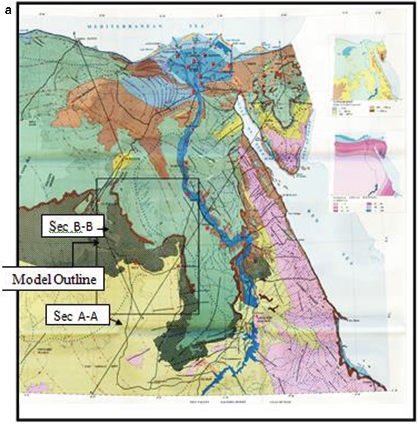
(a) Hydrogeological map of Egypt by RIGW [13] showing the study area. (b) Cross section A-A through the study area. (c) Cross section B-B through the study area

5 Numerical Simulation of the Study Area

5.1 Hydrologic Setting of the Study Area Model

The study area behavior of the aquifer system is acquired mainly from the hydrogeological map and other reports and papers available about the Nubian Aquifer system. It must be noted that CEDARE Report 2002 will be considered as the main source of data in this study. The modeling was carried out as follows:

In order to have more confidence in the hydrologic parameters GIS with Visual Basics model is used in order to fill the gaps in those parameters needed for the Nubian main model. Each Oasis will have a separate local model [14].
A second model is set for the entire model domain using the MODFLOW model software. The objective of the second model is to set the required aquifer boundary conditions.
Upon setting the model properties and its boundary conditions from the last models, a third final model domain was furnished including all wells replacement until the year 2010 and their discharges. It must be noted that water supply wells are added to the final model in order to have an actual groundwater management plan.
At this stage, simulating the development of the different scenarios is followed for the prediction of the related aquifer response using the latest well groups. The model will run for 100 years (2010–2110) in order to set the future water management plan for the three Oases.

5.2 Mathematical Formulation (Governing Equations)

The Governing equation that suits the Nubian confined aquifer is the two-dimensional groundwater partial differential equation as given below:

$\partial \left({T}_{\mathrm{xx}}\frac{\partial h}{\partial x}\right)+\partial \left({T}_{\mathrm{yy}}\frac{\partial h}{\partial y}\right)+Q=S\frac{\partial h}{\partial t}$

(1)

where the transmissivity and the horizontal conductivity (HC) are defined as follows:

T _xx = K _xx × Saturated thickness of layer in x direction (L²/T)
T _yy = K _yy × Saturated thickness of layer in y direction… (L²/T)

And the storage coefficient S is given as:

S = S _s × Saturated thickness of layer
K _xx, K _yy (L/T) are values of the hydraulic conductivity along the horizontal principal axes in the layer. In case of the Nubian aquifer, it was found from many research works and CEDARE Report that almost the horizontal HC K _xx = K _yy = K
S _s is the specific storage coefficient of the aquifer (L⁻¹)
h is the piezometric head at any point in the model domain (L)
Q is the pumping rate in the model (L³/T)
S _y is the specific yield or effective porosity of the unconfined aquifer.

On the other hand, for the unconfined aquifer, the three-dimensional groundwater flow equation becomes:

$\frac{\partial }{\partial x}\left({K}_{\mathrm{xx}}\frac{\partial h}{\partial x}\right)+\frac{\partial }{\partial y}\left({K}_{\mathrm{yy}}\frac{\partial h}{\partial y}\right)+\frac{\partial }{\partial z}\left({K}_z\frac{\partial h}{\partial z}\right)+Q={S}_y\frac{\partial h}{\partial t}$

(2)

where z is the third dimension and K _z is the vertical hydraulic conductivity.

5.3 The Model Package of the MODFLOW

Visual MODFLOW model is the software package developed by Waterloo Hydro-geological Inc. It is used to solve three- or two-dimensional groundwater flow and contaminant transport simulations with the finite difference approach.

This package combines MODFLOW and MT3D with the most intuitive and powerful graphical interface available.

The logical menu structure and easy to use graphical tools allow the following:

Dimensioning the model domain and selecting units.
Conveniently assigning model properties and boundary conditions.
Running the model simulations.
Calibrating the model using manual or automated techniques.
Optimizing the pumping well rates and locations.
Visualizing the results using 2D or 3D graphics.

The MODFLOW software used the finite difference approach for its simulation principles. Complete explanations about using the finite difference techniques are given in [9].

5.4 Procedures for MODFLOW Implementation

5.4.1 The Model Domain

As explained, the extent of the model domain for the Dakhla Basin covers an area between longitudes (27° E and 31.5° E) and between latitudes (24° N and 28° N). Since the MODFLOW supports only both the foot unit and the metric unit systems. Therefore, the metric unit system is used in our model domain. The model dimensions, therefore cover 440 × 460 km. The shorter lengths are the eastern and western boundaries of the model parallel to longitudes 27° E and 31.5° E, respectively. On the other hand, the longer lengths are located at the southern and northern boundaries of the model parallel to the latitudes 24° N and 28° N, respectively. The model grid has a uniform cell size all over the model domain. The cell size of 4 × 4 km was found suitable for the problem at hand. The model grid, in this case, will have 115 columns and 110 rows. The model coordinate systems related to the geographical coordinates are given in Table 2. It must be remembered that the model domain was drawn on Google earth. An error of 4% was found between the coordinates obtained from both the hydrological map and the Google Earth data. This error is considered agreeable to all geological survey Departments.

Table 2

Relation between (geographical) and model coordinates

Coordinates	Geographical coordinates	Model dimension in m
X _min	At Long 27° E	0
Y _min	At Lat 24° N	0
X _max	At Long 31.5° E	460,000
Y _max	At Lat 28° N	440,000

The model origin (0,0) is located, therefore, at the intersection of Long. 27° E and Lat 24° N

According to the conceptual model, the MODFLOW model will have two zones. The model first zone will simulate the depleting limestone layer and the nonconductive shale layer. The model second zone will simulate the main and productive Nubian aquifer. It is a deep aquifer where its lower surface boundary is located at the basement complex surface. The model thickness will simulate the actual vertical thickness which is between the maximum ground surface elevation (little less than 700 m (amsl)) and the minimum elevation of −3,300 m (bmsl) at the basement complex surface boundary.

By placing the three surfaces, the upper ground surface, the intermediate boundary surface, and the basement complex surface using the MODFLOW processing the model domain can be formulated. Figures 4, 5, and 6 show the plan of the ground surface contours, the intermediate surface contours, and the basement complex surface boundary contours. Figure 7 shows an intermediate cross section through Dakhla Oasis in the model domain located at Lat 26° N at a distance Y = 220,000 m from the model origin.

../images/437178_1_En_62_Chapter/437178_1_En_62_Fig4_HTML.png — Fig. 4
Topographical map of the model area

../images/437178_1_En_62_Chapter/437178_1_En_62_Fig5_HTML.png — Fig. 5
Contour lines of zone 1 bottom

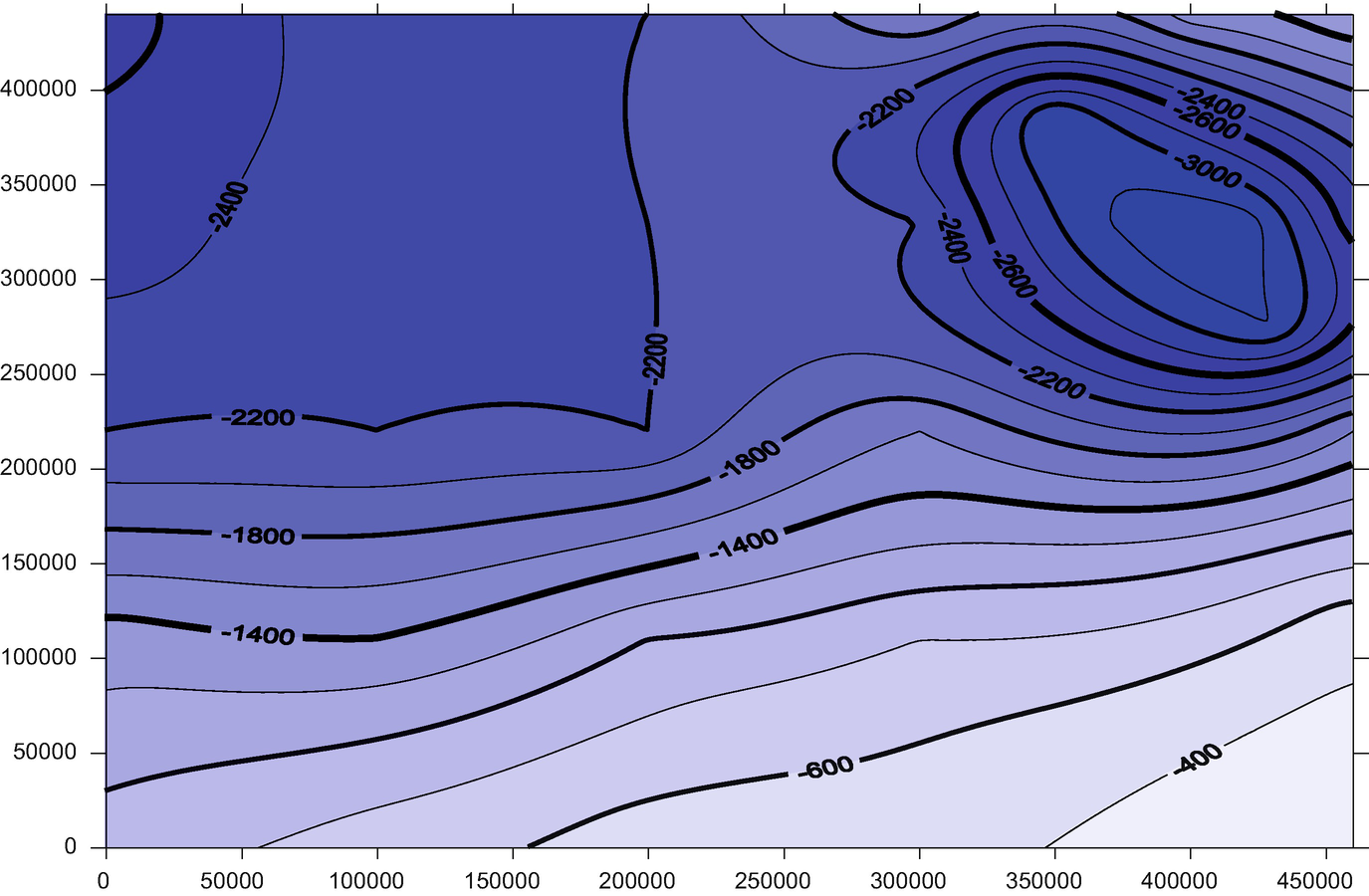
../images/437178_1_En_62_Chapter/437178_1_En_62_Fig6_HTML.png — Fig. 6
Basement complex bottom layer 2

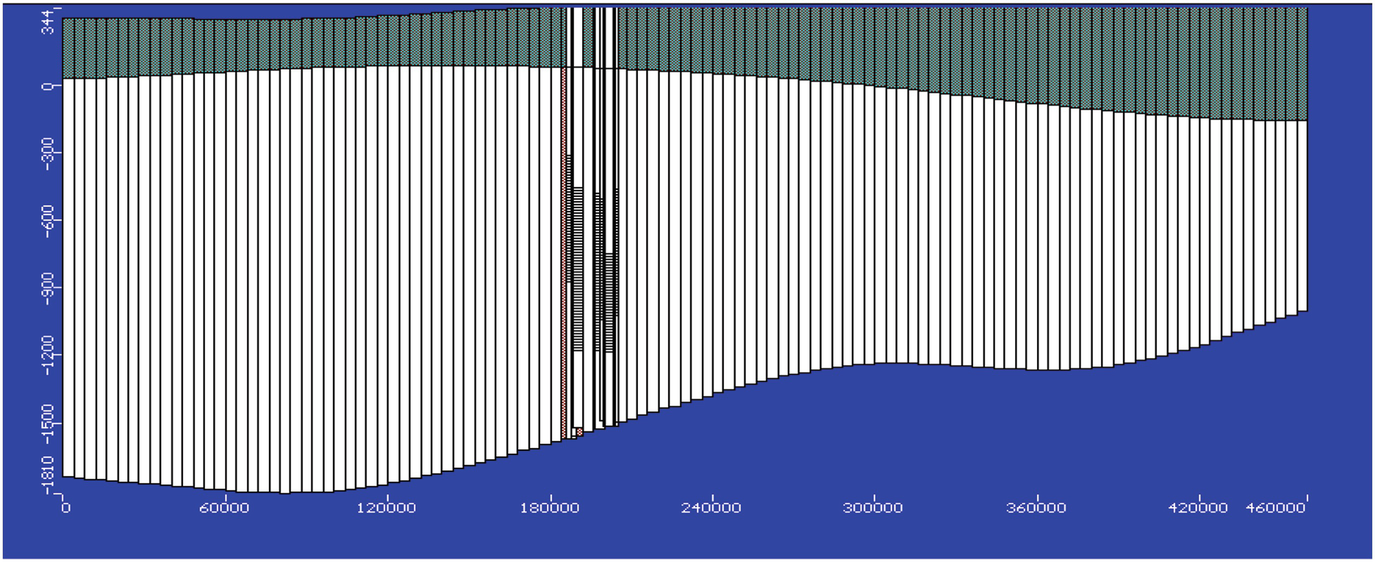
../images/437178_1_En_62_Chapter/437178_1_En_62_Fig7_HTML.png — Fig. 7
Cross section through the middle of the model domain at Dakhla Oasis (through Lat 26° N) with distance y = 220,000 m from the origin

5.4.2 Model Properties

The model properties include the hydraulic conductivity (HC), storage or specific storage coefficient (S _s), and the initial head. Specific storage (1/L) will be used. In spite of the several pumping tests that were done in the three Oases as given in Table 3 (obtained from CEDARE report), yet some data for S _s are missing. This can be overcome by using local models and in the same time adjusting the available data for the model properties. A regional calibration model which includes the entire Oasis together using the MODFLOW model would adjust the boundary conditions.

Table 3

Average hydraulic parameters of the Nubian Aquifer System (refer to CEDARE Report [15])

Region	No of Pumping tests	Saturated thickness (m)	Transmissivity (m²/s)	Hydraulic cond. (HC) (m/s)	Storage coefficient(s) (S)
Farafra	8	2,600	1.20E-02	5.4 × 10⁻⁵	?
Abu minqar	3	2,500	5.469E-02	2.18 × 10⁻⁴	?
Dakhla	21	1,850	1.1E-02	6.1E-05	6.35 × 10⁻⁴
Kharga	59	1,280	5.9E-03	2.90E-05	2.84 × 10⁻⁴

Note: ? = missing data in CEDARE Report. All missing data was achieved by VB-GIS model as stated in the literature

5.5 Local Models

In this research work, the local models were used to further adjust both HC and S _s and find any missing data as S _s. The method used for adjustment of both properties is by using the GIS with the visual basic model which was achieved by Gad and Soliman [14]. The method was used for adjustment or calibration process of both the HC and S _s.

The adjustment started by using data shown in Table 3 of HC and S (obtained by CEDARE from pumping tests [6]) and comparing it with calculated data from the drawdown by Eq. (3). This equation was introduced to the data code of the visual basic (VB) which is in the GIS extension tool. Upon getting the drawdown values for the entire wells at selected network stations obtained by the VB, the GIS can draw the drawdown contours through the spatial analyst in the GIS tools as given below.

Table 4 which was obtained by CEDARE includes the number of pumping tests in each Oasis, the average aquifer thicknesses, the HC, and the storativity for each Oasis. Table 5 shows the total optimum discharges for each Oasis for specific years that was optimized by CEDARE model (Fig. 8), which was also developed by CEDARE and was helpful in getting the relation between the piezometric head with respect to time in years for the observed wells in the three Oases. This figure was helpful to extract the observed drawdown at the shown wells for a selected short period with its related discharges. The reason for selecting the short periods with the local models is to try to get the zero drawdown in each Oasis as shown in the following sections. The GIS method follows the following steps:

1.
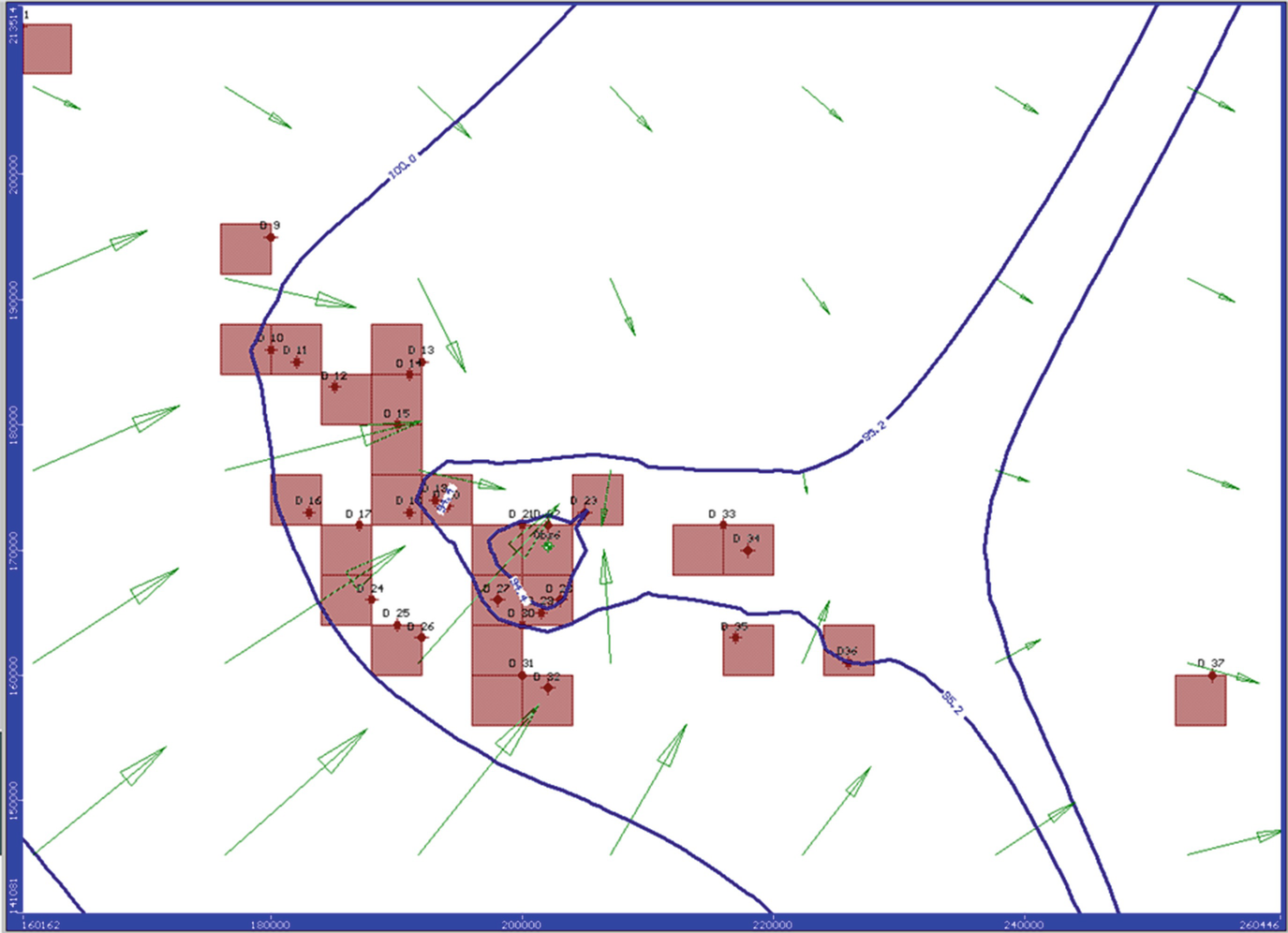
Locate first the well group for each Oasis in a point shapefile using the selected coordinates in model domain as shown in Figs. 29, 30, and 31 in Appendix 1
2.
Once the well groups were located, and the well discharges are assigned to each well then the Visual Basic Code (VB Code) is designed to make a grid of points to stand for the observation points using the same coordinates of the well groups. There will be two coordinate systems (xw, yw)_i for the well (i) and other coordinates for the observation points (xp, yp)_k (i for the well number and k for the grid point number).

In order to calculate the drawdown at any grid or observation point, Modified Theis Equation is used in VB Code as,

Table 4

New Valley extractions (1998–2010) (CEDARE Report [15])

Area	1998		2000		2005		2010
Area	m³/s	Mm³/year	m³/s	Mm³/year	m³/s	Mm³/year	m³/s	Mm³/year
Farafra	5.05	159	2.85	90	3.5	110	4.5	142
Dakhla	8.75	276	8.75	276	10.3	325	11.85	374
Kharga	3.96	125	3.96	125	3.96	125	5.00	158

Table 5

Drawdowns (DD) calculated and observed for Farafra parameters

Oasis name	Q (m³/s)	Observation well locations	Pumping time	Model DD (m)	Observed DD (m)	Note
Farafra	2.85	NF9 (Obs1)	5 years (1995–2000)	2.8	2.5	Av error 6.5%
	3.5	X = 60,000 m	5 years (2005–2010)	3.8	3.4	Av error 6.5%
		X = 60,000 m				K = 5 m/day
		Y = 308,000 m				S _s = 2.00E-05
	5.05
	5.05		10 years (1990–2000)	6.4	6.2

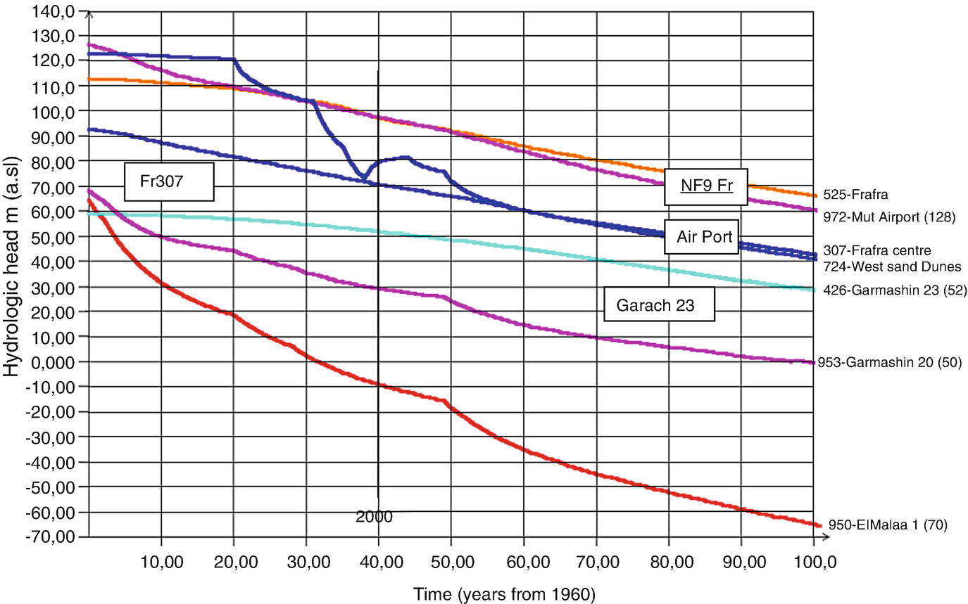Note: The data for Q and observed drawdown (DD) at Obs1 were obtained from Fig. 9 and Table 4 which were adopted from CEDARE Report

../images/437178_1_En_62_Chapter/437178_1_En_62_Fig8_HTML.png — Fig. 8
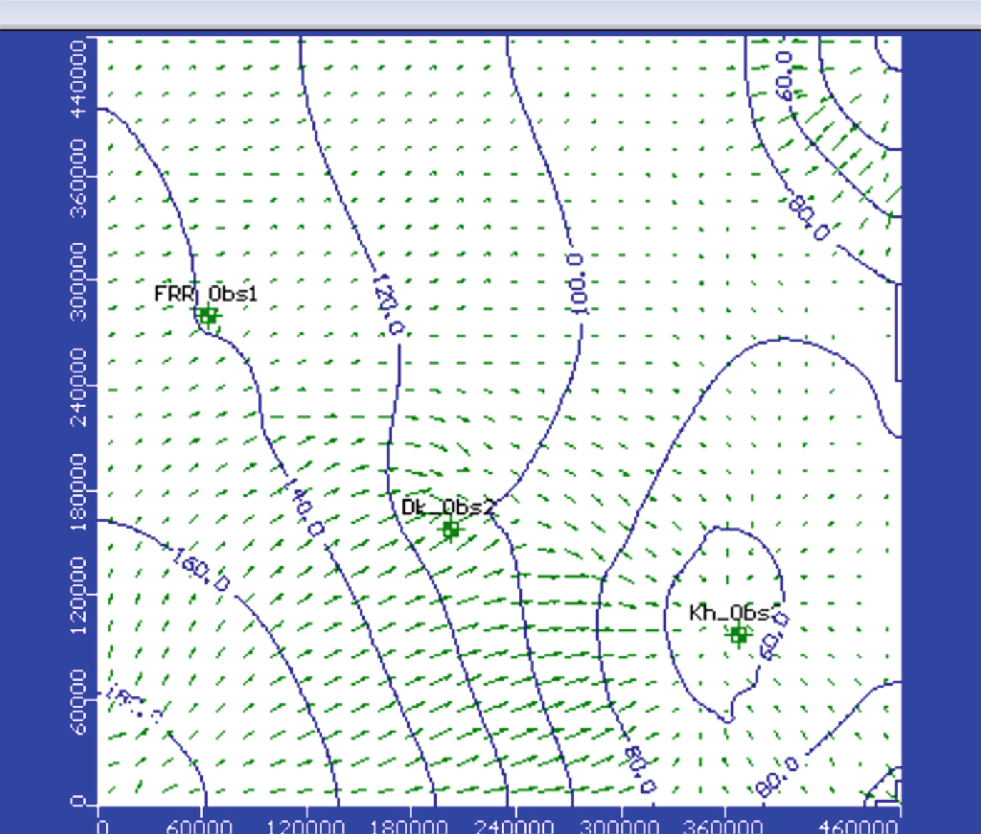
Piezometric head at various locations of wells at the New Valley [2]

${d}_k=\left(2.3{Q}_i/4 T\pi \right)\left[\log \left(2.25 Tt/{R_i}^2S\right)\right]$

(3)

where

d _k = drawdown at an observation point k (m)

Q _i = well discharge for well i (m³/day)

T = average transmissivity of the aquifer = K – Saturated aquifer thickness of the selected Oasis as given in Table 5 (m²/day)

K = the hydraulic conductivity (HC) (m/day) of the Oasis

t = selected pumping time in days

R _i = the distance between the well (i), and the observation point (k) =[(x(k) − x(i))² + (y(k) − y(i))²]^0.5

4.
For each well the drawdown was calculated and summed at each observation point k. This was obtained by VB code and located at the respective point. It must be noted that any observation point located at any well is discarded by the Code. The GIS will then draw the drawdown contours as shown for the three Oases (Figs. 9, 11, and 13). Notice that the drawdown zero contours were located inside the Oases boundaries. This condition was found in this respect when the pumping time will not exceed 10 years for any Oasis in order to prevent any groundwater interference between Oases. Figures 29, 30, and 31 in Appendix 1 give both Geographic coordinates and the model coordinates system for each well at Farafra, Dakhla, and Kharga Oases, respectively.
5.
The adjustment process started by selecting the drawdown values for one or two wells near the center of each Oasis. Then compare the results with the observed and calculated values as mentioned before. In this research, it was found that Storage Coefficient S was much more sensitive on the drawdown than the H.C. K, so S _s was selected in the calculations for its variation to try to narrow the gaps between both observed and calculated drawdown values (Figs. 9, 10, 11, 12, 13, and 14).
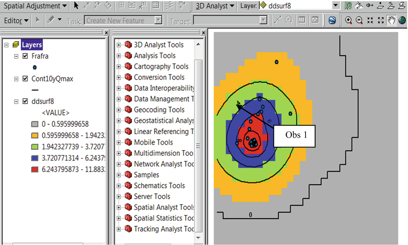Fig. 9
Drawdown contours for Farafra. Total Q = 5.05 m³/s run for a maximum period of 10 year as given in Table 5

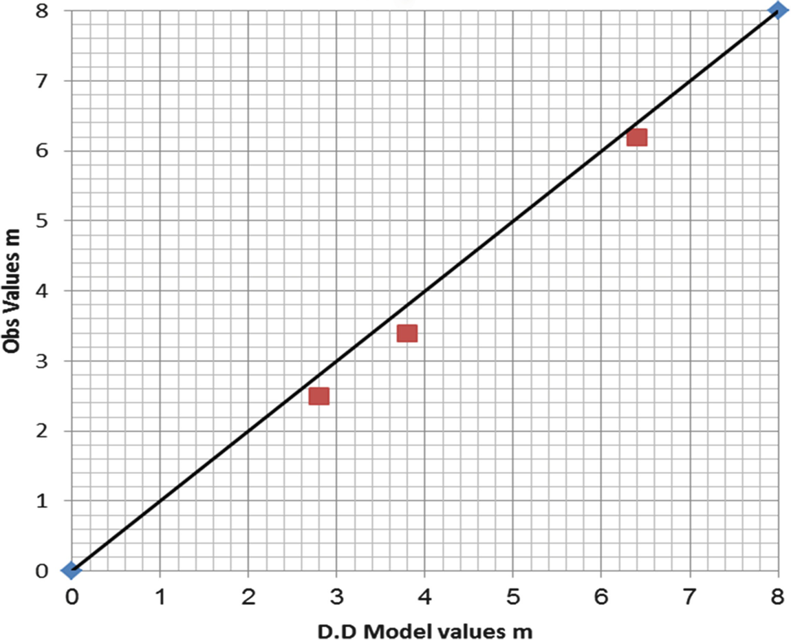Fig. 10
Farafra aquifer correlation values (refer to Table 5)

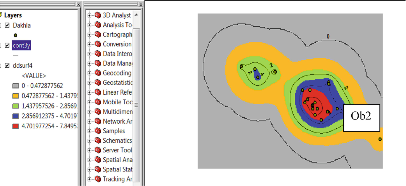Fig. 11
Drawdown contours of Dakhla Oasis using GIS and VBC (observation well locations Obs2 is at Mut airport)

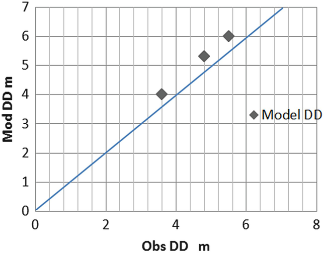Fig. 12
Relations between observed and model data for DD in Dakhla Oasis. See for observed well locations Obs2

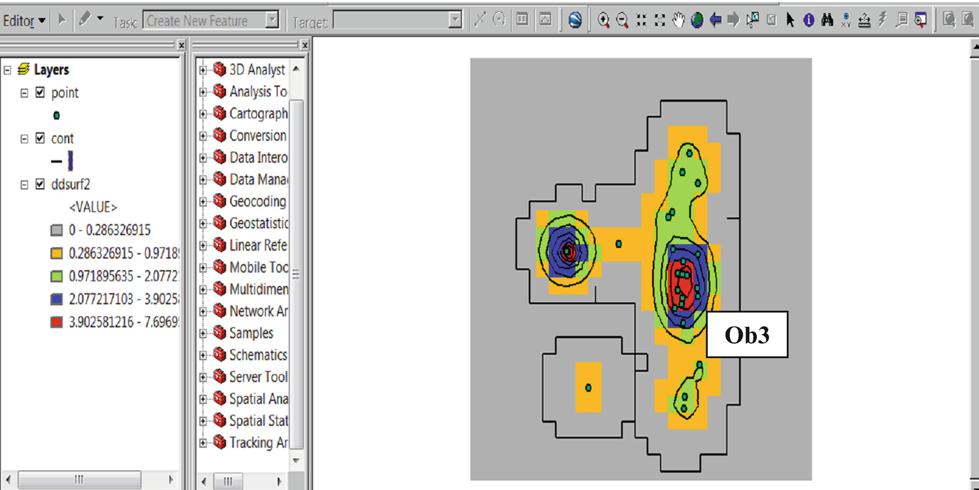Fig. 13
Drawdown for 5Y contours for Kharga (Obs3 stands for well observation 3)

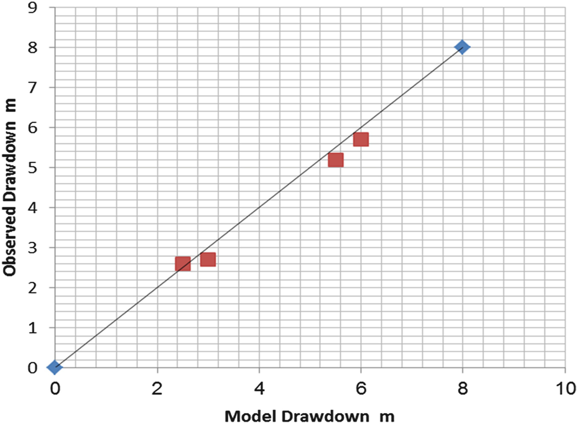Fig. 14
Kharga Oasis Parameter adjustment

Tables 5, 6, and 7 include the three observation well locations used for correlations and the results after the adjustment processing. Figures 10, 12, and 14 show the correlations between the observed and the calculated drawdown.

Table 6

Drawdowns (DD) calculated and observed for Dakhla Parameters

Oasis	Observation well with its model coordinates	Q (m³/s)	Pumping time	Model DD (m)	Observed DD (m)	Note
Dakhla	Airport Mut (Obs2)	10.3	5 years (2005–2010)	6.0	5.5	Av error 5%
	X = 200,170 m	10.3	3 years (2005–2008)	4	3.6	K = 8 m/day
	Y = 156,354 m	8.75	5 years (2000–2005)	5.3	4.8	S _s 8.00E-06

Note: The data of Q and observed drawdown (DD) were obtained from Fig. 8 which were adopted from CEDARE Report

Table 7

Drawdowns (DD) calculated and observed for Kharga Parameters

Oasis name	Q (m³/s)	Observation well with its model coordinates	Pumping time	Model DD (m)	Observed DD (m)	Note
Kharga	3.96	Garmashin 23 (Obs 3) X = 360,900 m Y = 104,600 m	5 years (2000–2005)	3	2.7	Av error 7.5% K = 3.25 m/day S _s = 2.40E-05
		Garmashin 23 (Obs 3) X = 360,900 m Y = 104,600 m	10 years (2000–2010)	6	5.7
		Garmashin 20 (Obs4) X = 362,000 m Y = 93,170 m	5 years (2000–2005)	2.5	2.6
		Garmashin 20 (Obs4) X = 362,000 m Y = 93,170 m	10 years (2000–2010)	5.5	5.2

Note: The data of Q and observed drawdown (DD) were obtained from Fig. 8 which were adopted from CEDARE Report

Regarding the local models of the three Oases, one can state that the difference between the HC values obtained by the GIS/VB and CEDARE values is close. However, the storativity values were adjusted, and the missing storage values were obtained. For this reason, Soliman [12] found that the local model results gave more confidence in the obtained model properties. However, a regional model for the three Oases is set to calibrate the model boundary conditions.

5.6 Regional Model

5.6.1 Model Preparations

The hydraulic conductivity and specific storage adjustments using the GIS with the Visual Basic extension program were found successfully for each Oasis. The regional model using the MODFLOW domain was built particularly for the calibration stage in order to adjust the model boundary conditions. The model domain would contain the well network and its discharges for the period of years (2000–2020). The well discharges are as given in Table 4 which was obtained from CEDARE Report. The well network location is found in Figs. 29, 30, and 31 in Appendix 1.

The initial head needed for the model as given in Fig. 15 was adopted from the hydrogeological map obtained by RIGW 1999/2000. Three observation wells (vis Obs1, Obs2, and Obs3) were selected for calibration process, one observation well in each Oasis.

../images/437178_1_En_62_Chapter/437178_1_En_62_Fig15_HTML.png — Fig. 15
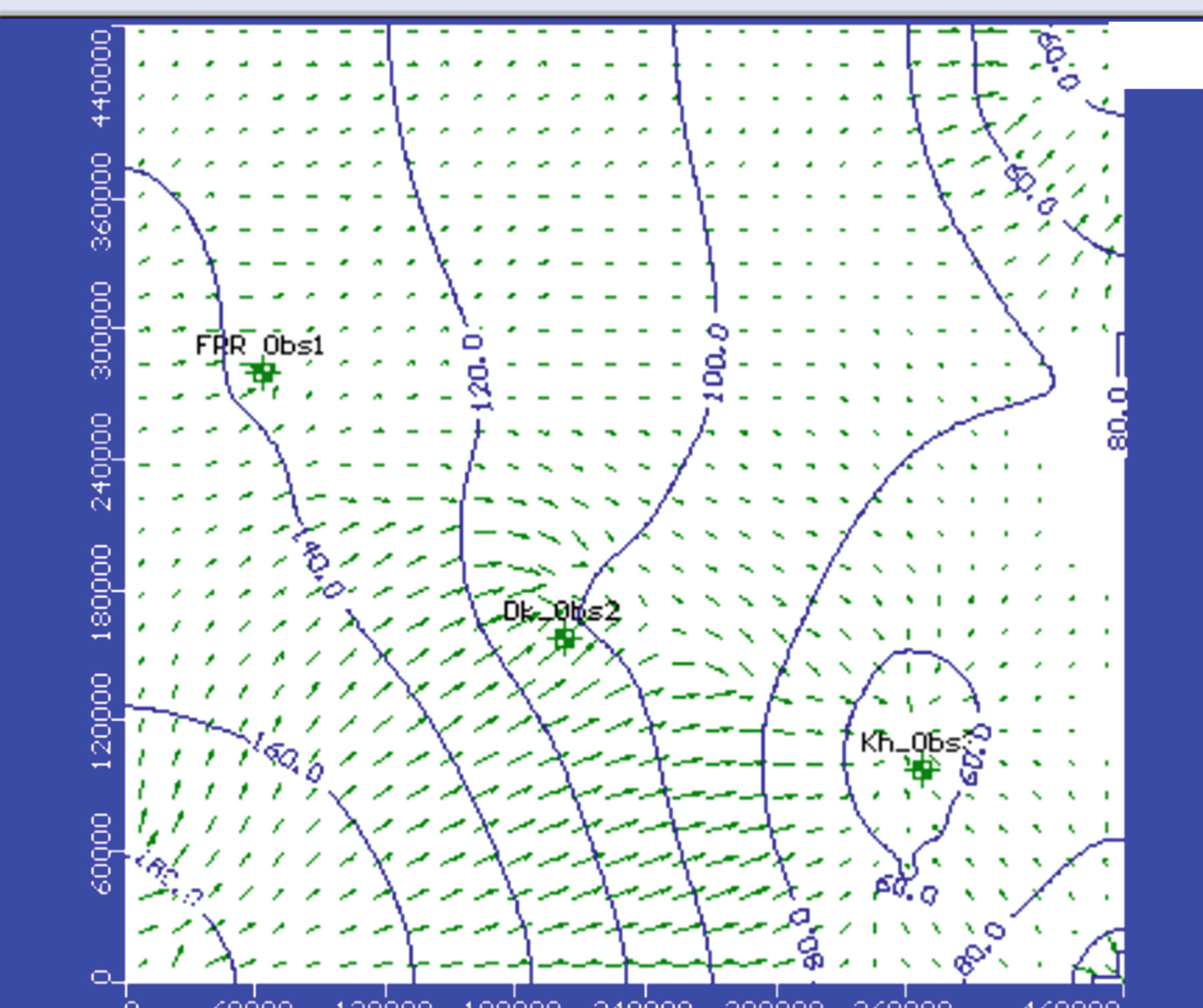
Initial head contours for Dakhla Basin developed from the Hydrogeological Map by RIGW

Those wells are chosen to fit the drawdown data in Fig. 8 and as located in the GIS model. The benefit of using this stage is also to get the piezometric head at year 2010 which will be used in the final model as its initial head. Table 8 gave the final adjustment for model properties resulted from the local models. Those values were distributed in the model domain as given in Figs. 16 and 17.

Table 8

The final adjusted values for model properties

Location	S _s (1/L)	K (cm/s)
Farafra	2.00E-05	6.00E-05
Dakhla	8.00E-06	8.00E-05
Kharga	2.40E-05	4.00E-05

../images/437178_1_En_62_Chapter/437178_1_En_62_Fig16_HTML.png — Fig. 16
HC > distribution in the model domain

../images/437178_1_En_62_Chapter/437178_1_En_62_Fig17_HTML.png — Fig. 17
Specific storage distribution in the model domain

5.6.2 Boundary Conditions

As a first glance to the model area, the boundary of Assiut Governorate area at the upper eastern corner of the model domain can be taken as a constant head boundary due to the presence of some seepage flow as reported by the groundwater Institute in this location. This boundary is also formed from series of faults between the Nile Basin alluvial material and the Nubian aquifer as seen in Fig. 3b. In spite of both aquifers are different from each other, yet there is a possibility that both aquifers are hydraulically connected as reported also by the groundwater Institute in this location.

Since the groundwater level fluctuates around 50 m (amsl) in Assiut alluvial aquifer, therefore a constant head boundary of 50 m can be taken at the Nile Basin boundary at north east of the model domain.

Upon looking at the initial head map, two other sources of boundaries may be postulated. These are the southwestern corner (BC2) and the southeastern corner (BC3) of the model domain (Fig. 21 where more details are given). The rest of the model boundaries are approximated as flow lines.

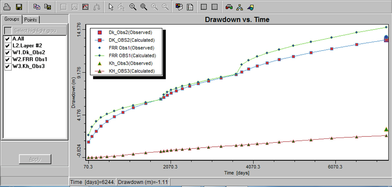
The aforementioned boundary conditions were slightly increased or decreased cell by cell several times until successful calibration or an optimum condition gave 95% confidence as given in Figs. 18 and 19. Those figures were obtained from the model output for 20-year period (year 2000 to year 2020) as given in Fig. 20.

../images/437178_1_En_62_Chapter/437178_1_En_62_Fig18_HTML.png — Fig. 18
DD vs time at the tutee Oasis

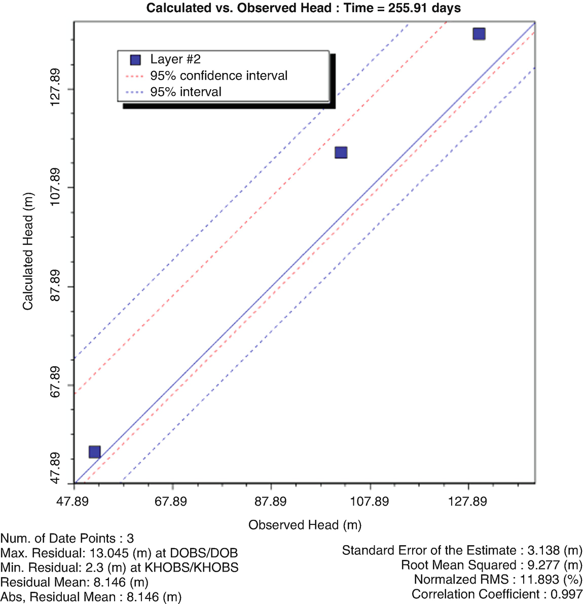
../images/437178_1_En_62_Chapter/437178_1_En_62_Fig19_HTML.png — Fig. 19
Calculated vs observed head at the observed wells in the three Oases. The observed data is from CEDARE drawdown data

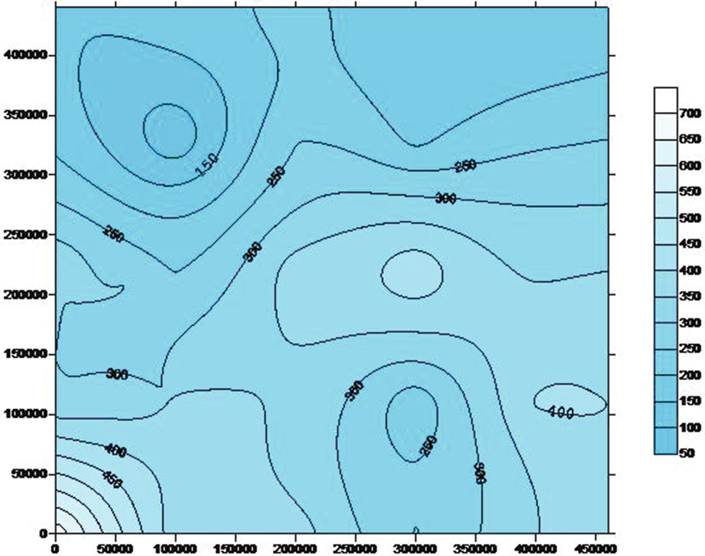
../images/437178_1_En_62_Chapter/437178_1_En_62_Fig20_HTML.png — Fig. 20
Piezometric head map at 2020 resulted from the calibration process

Figure 21 shows the observation wells, the final boundary condition after calibration, and the initial head at the year 2000 as given below:

1.
For observation well coordinates (Far obs1), (D obs2), and (Kh obs3) see Tables 5, 6, and 7.
2.
Boundary condition BC1 is set at the Nile Basin boundary south of Asyut Governorate as mentioned before.
3.
Boundary conditions BC2 and BC3 which took L section are set as follows:
1. (a)
  The number of cells of BC2 = 11 cells in the vertical direction and 8 cells in the horizontal direction. The average potential head was found from the calibration trials to be 180 m (amsl)
2. (b)
  Also from the calibration trials, the L section BC3 boundary was found to have four vertical cells and three horizontal cells. The average head value was also found to be =75 m (amsl) resulted from the calibration process.

../images/437178_1_En_62_Chapter/437178_1_En_62_Fig21_HTML.png — Fig. 21
Initial head in the year 2000, boundary conditions and the three observation wells used in the model domain

Figure 22 shows the potential head at the year 2010 which was selected to be the initial head for the final model.

../images/437178_1_En_62_Chapter/437178_1_En_62_Fig22_HTML.png — Fig. 22
Piezometric head map at year 2010 used as initial head of final model and showing also the three observation well locations

5.7 Final Model and Analysis

The final model domain is arranged to include all the wells which were replaced and constructed recently (September 2010) in the three Oases. Most of the new wells were drilled during 2008–2010. The boundary condition was already installed as mentioned in the regional model study.

Tables 9, 10, and 11 (see Appendix 2) include all the wells and its locations that have been obtained from the Groundwater Sector in the Ministry of Water Resources and Irrigation. It must be noted that all the water supply wells were also included in the tables. Two scenarios are adopted to run the final model as given below.

Scenario 1

In order to study the groundwater management in Dakhla Basin, an optimization study should be done. The optimization procedure of the Groundwater Sector of the Ministry of Irrigation is used. The process first of all deals with the Nubian aquifer in Dakhla Basin as a nonrenewable groundwater reservoir.

In this kind of aquifer, groundwater development should follow the groundwater mining system rules. This means that any groundwater exploitation should postulate constrictions for development. The Groundwater Sector of the Ministry adopted the main constriction in the groundwater management plan is that the maximum drawdown of any well field in such kind of aquifer should not be greater than 60 m resulted from running the pumping wells for 100-year period plus the historical drawdown value that exists before the 100 year period. This postulation took mainly into consideration the economic and the timescale factors. The timescale factor is postulated to have the 100-year period as enough to investigate for an additional water resources system to cover the lack of the water requirement of the area.

The final model was run first for the 100-year period (from the year 2010 to 2110) in order to find the maximum drawdown for each Oasis. The second step was to find the historical drawdown before the year 2010. Figure 8 developed by CEDARE was used to get the historical drawdown for the period between the year 1960 (the time at which the New Valley project started) and the year 2010. The three wells that were selected to find the historical drawdown for the three Oases are

Well number 307 in Farafra was used to get the historical drawdown for Farafra Oasis.
Well Mut Airport was used to get the historical drawdown for Dakhla Oasis.
Garmashine well 23 was used to get the historical drawdown for Kharga Oasis.

Figure 23 shows the final model results of the head contours in the model area at the year 2110. The total drawdown for the same period is given in Fig. 24. Notice in the figure the zero drawdown contours separates the Khrga Oasis well field from both Farafra and Dakhla Oases well fields.

../images/437178_1_En_62_Chapter/437178_1_En_62_Fig23_HTML.png — Fig. 23
Model outcome of head contours of 100-year period

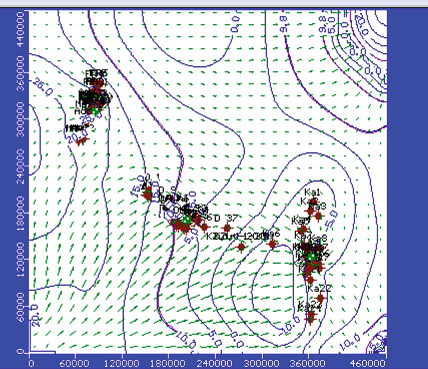
../images/437178_1_En_62_Chapter/437178_1_En_62_Fig24_HTML.png — Fig. 24
Drawdown contours for 100-year period

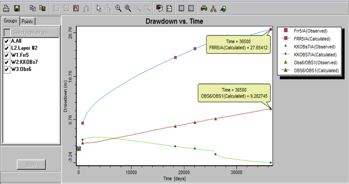
Notice also that the drawdown in Kharga Oasis is denoted by negative sign since it is below zero drawdown line. On the other hand, Fig. 25 shows the drawdown as recorded by the observation wells. It is clear from the figure that Farafra Oasis gave the highest drawdown. Figure 26 shows the maximum and minimum drawdown values obtained by the MODFLOW. It also gave an absolute drawdown of 55 m for the model area of Dakhla Basin.

../images/437178_1_En_62_Chapter/437178_1_En_62_Fig25_HTML.png — Fig. 25
Drawdown vs time at the three observation wells in the three Oases

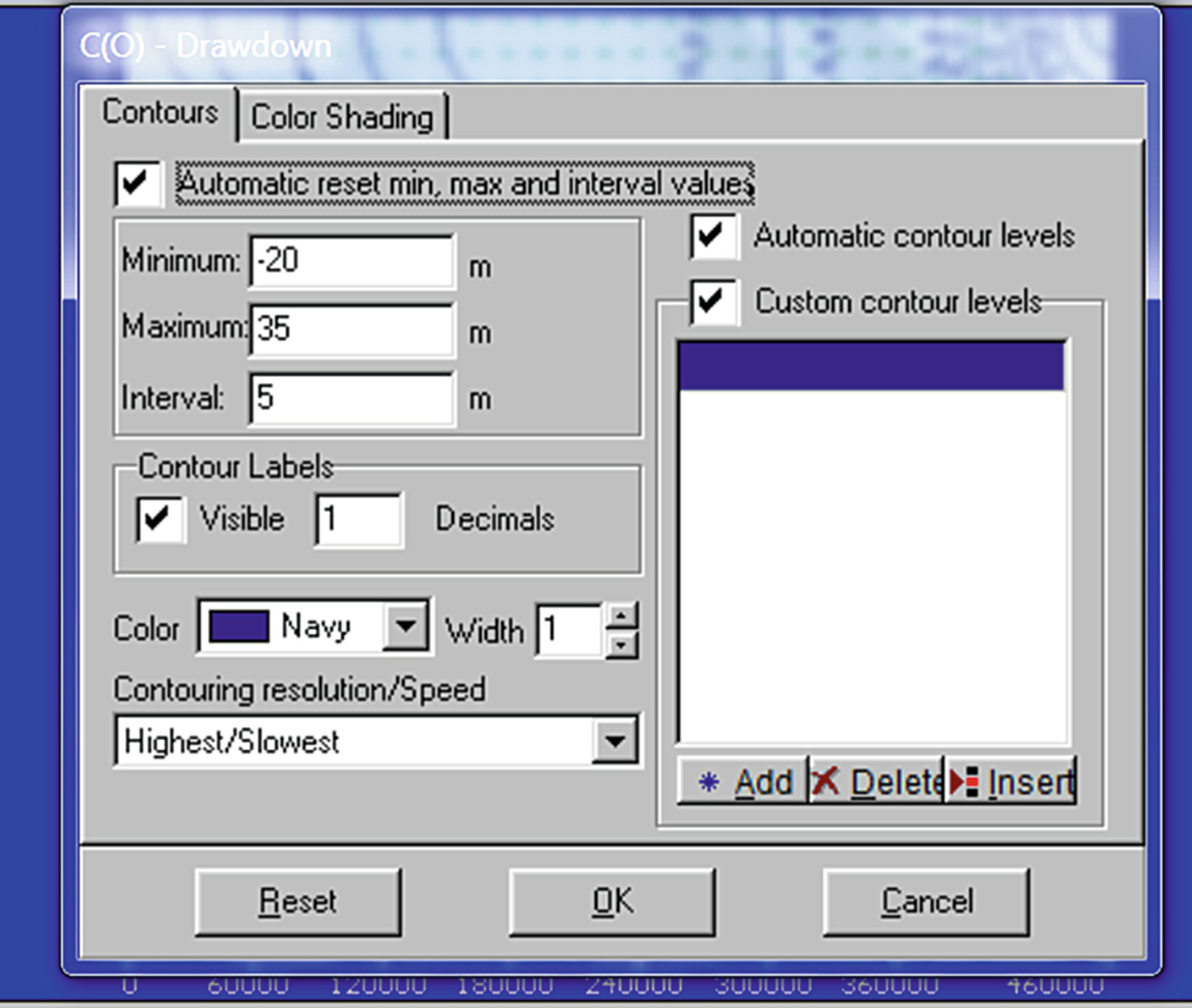
../images/437178_1_En_62_Chapter/437178_1_En_62_Fig26_HTML.png — Fig. 26
Maximum and minimum drawdowns at the year 2110

The value of drawdown −20 m denotes the maximum drawdown in Kharga Oasis whereas the drawdown value of 35 m denotes the maximum drawdown near Farafra area. The negative sign in the drawdown was only denoted algebraically by the model. This is also due to the presence of the 0.0 drawdown contour where any value above 0.0 is positive, and any value below 0.0 is negative. The 0.0 contour can be resembled by an island encountered by water, postulated as 0.0 level, and any drawdown inside the island is considered as having a negative value. It can be noticed that the flow inside the 0.0 contour approaches the steady state condition.

This can be visualized by subtracting the piezometric head in the year 2010 minus the piezometric head at the year 2110. The reason for that is due to the reduction of the well discharges in Dakhla Oasis in the year 2010 by 50% as given in Table 10 in Appendix 2. The model study considered this reduction until the year 2110.

According to optimization procedure for Kharga Oasis the maximum drawdown was found to be 20 m in 100-year period. The historical drawdown value started from the year 1960 which was considered as the beginning of New Valley development may be adopted from Fig. 8.

The Garmashine well 23 in Fig. 8 (see its location in Fig. 31 in Appendix 1) was used to give the historical drawdown. This value was found to be 42 m.

Therefore, the total drawdown in this respect until the year 2110 would be 62 m which is considered as critical drawdown value by the Ministry of Irrigation optimization process.

The historical drawdown in Farafra Oasis using Well 307-Farafra gave 26 m (see Fig. 8). On the other hand, the 100-year maximum drawdown in Farafra was found to be 35 m (Fig. 26). Therefore, the total drawdown became 61 m which do not favor any discharge increase. This is according to the Groundwater Sector postulation as mentioned before.

Concerning Dakhla Oasis, the 100-year maximum drawdown was found to be 24 m (Fig. 24). On the other hand, the historical drawdown of Mut Air port well gave 34 m. Accordingly, the total drawdown gave 58 m. Therefore, Dakhla Oasis allows further expansion which is discussed in the Scenario 2.

Scenario 2

In this scenario, the final model was run with higher discharge for Dakhla Oasis than that in Scenario 1. This was proved possible since the total maximum drawdown of Dakhla Oasis was found to be 58 m which is less than the critical drawdown (60 m as mentioned before). However, one should be very cautious to the well discharge increase. After a series of trials 15% increase of the well discharge (Q) was found reasonable in Dakhla Oasis. Figure 27 shows the expected piezometric head at the year 2110 with the increased well discharge. The new well discharges for Dakhla Oasis are also given in Table 10 in Appendix 2.

../images/437178_1_En_62_Chapter/437178_1_En_62_Fig27_HTML.png — Fig. 27
Piezometric head map of the model output at the year 2110 after increasing the well discharge by 15%

In order to calculate the maximum drawdown in Dakhla Oasis in this scenario, the piezometric map of Fig. 27 was zoomed near the center of the Oasis as given in Fig. 28 which gave the lowest contour value as 94.4 m. The initial contour that was passing through this area as given in Fig. 22 is 120 m. Therefore the drawdown in Dakhla center would be 25.6 m. Accordingly, by adding 25.6 m to the historical drawdown found in Scenario 1 of 34 m resulted total maximum drawdown of 59.6 m which considered safe and little less than critical drawdown. This fact should be taken into consideration when discharge increase for Dakhla basin development is planned.

../images/437178_1_En_62_Chapter/437178_1_En_62_Fig28_HTML.png — Fig. 28
Zooming of piezometric head map of Fig. 24 at Dakhla Oasis Center

6 Conclusions

The study area in this research is located in the middle part of Egypt’s Western Desert. It lies between latitudes 24°–28°^.N and longitudes of 27°–31.5° E. It includes the three Oases, Farafra, Dakhla, and Kharga, which are part of the New Valley area. It covers an area of about 440 km long by 460 km wide. It is equivalent to an area of 202,400 km² which is named as the Dakhla Basin. The western limestone plateau bound it to the east and north of Kharga and Dakhla region.

The main objective of this research is to evaluate the groundwater resources and its potentiality for development in the study area. The aquifer of this groundwater resource is mainly the deep Nubian Sandstone Aquifer which is located in the three Oases. Due to the scarcity of the groundwater recharge in the Nubian aquifer, it is hydrogeologically treated as groundwater mining aquifer [12].

Three groundwater models were used in this respect. A local model using GIS accompanied by the visual basic was first prepared to adjust the model properties. A second model using MODFLOW was furnished to calibrate the boundary conditions of the main model. The third model was using the main model as a final model to find the main objectives which are the groundwater potentiality and its management in Dakhla Basin The model was run for a 100-year period to suit the groundwater mining conditions.

As an outcome of the model study for the optimum management strategy in Dakhla Basin, two scenarios were postulated. The objective is to maintain the resultant drawdown in the development areas within an acceptable range for economic purposes besides obtaining the most appropriate area for development in Dakhla Basin.

The salient fact from this study showed that Dakhla Oasis is the only place in the New Valley area where land reclamation development can safely take place.

Appendix 2

Table 9

Farafra well group for final Model

No		X (m)	Y (m)	Q (m³/day)
1	MZ1	88,000	312,000	13,300
2	MZ2	80,000	304,000	18,700
3	MZ3	81,000	311,000	17,050
4	Mz4	80,000	315,000	15,650
5	Mz5	86,000	311,000	18,000
6	Mz6	87,000	310,000	19,800
7	MZ7	85,000	308,000	18,000
8	MZ8	90,000	315,000	12,500
9	MZ9	90,000	319,000	8,900
10	MZ10	88,000	317,000	15,250
11	Mz11	83,500	306,000	18,000
12	MZ12	83,000	307,000	15,600
13	MZ13	84,000	310,000	17,000
14	MZ14	85,000	313,000	9,200
15	FR1	85,500	335,000	16,430
16	FR2	83,000	335,000	18,095
17	FR3	85,000	336,000	16,720
18	FR4	86,000	345,000	22,572
19	FR5	91,000	346,000	12,932
20	FR6	92,000	346,000	18,216
21	MNQ1	90,000	335,000	15,050
22	MINQ2	70,000	275,000	15,050
23	MNQ3	64,000	274,000	15,824
24	MNQ4	65,000	275,000	11,650
25	Add1	74,000	297,000	16,450
26	Add2	86,000	310,000	14,950
27	Add3	87,000	320,000	13,000
28	Add4	80,000	321,000	12,300
29	Add5	80,000	312,000	13,500
30	Add6	82,000	320,000	13,000
			Total (m³/day)	462,689
			Total (m³/s)	5.355197

Table 10

Dakhla well group for final model

No		Longitude	Latitude	X (m)	Y (m)	Q (m³/day)	1.15 × Q
1	Teneda1	29.250	25.455	225,000	160,000	12,407	14,268.05
2	Teneda2	29.260	25.464	226,000	161,000	11,874	13,655.1
3	Balat1	29.180	25.545	218,000	170,000	10,786	12,403.9
4	Balat2	29.170	25.482	217,000	163,000	8,581	9,868.15
5	Balat3	29.160	25.564	216,000	172,000	12,944	14,885.6
6	Asmant1	29.050	25.573	205,000	173,000	14,636	16,831.4
7	Masara1	29.020	25.564	202,000	172,000	14,947	17,189.05
8	Masara2	29.015	25.500	201,500	165,000	15,303	17,598.45
9	Shekwali	29.030	25.509	203,000	166,000	10,855	12,483.25
10	Mute1	28.900	25.491	190,000	164,000	11,678	13,429.7
11	Mute2	29.000	25.455	200,000	160,000	13,797	15,866.55
12	Mut3	29.020	25.445	202,000	159,000	12,906	14,841.9
13	Mut4	28.920	25.482	192,000	163,000	14,466	16,635.9
14	Mut5	29.000	25.491	200,000	164,000	14,465	16,634.75
15	Hend1	28.980	25.509	198,000	166,000	15,289	17,582.35
16	Owena1	29.000	25.564	200,000	172,000	16,176	18,602.4
17	Rashda1	28.910	25.573	191,000	173,000	16,382	18,839.3
18	Rashda2	28.930	25.582	193,000	174,000	17,196	19,775.4
19	Bedkhlo1	28.940	25.577	194,000	173,500	16,692	19,195.8
20	Kalamon1	28.880	25.509	188,000	166,000	15,570	17,905.5
21	ElGedida1	28.870	25.564	187,000	172,000	14,025	16,128.75
22	ElGedida2	28.830	25.573	183,000	173,000	15,526	17,854.9
23	Mosh1	28.900	25.636	190,000	180,000	16,544	19,025.6
24	Kasr1	28.910	25.673	191,000	184,000	17,960	20,654
25	Kasr2	28.920	25.682	192,000	185,000	14,856	17,084.4
26	Kasr3	28.850	25.664	185,000	183,000	16,844	19,370.6
27	Mawhub1	28.820	25.682	182,000	185,000	15,807	18,178.05
28	Mawhub2	28.800	25.691	180,000	186,000	15,507	17,833.05
29	Mawhub3	28.800	25.773	180,000	195,000	16,693	19,196.95
30	Mawhub4	28.550	25.864	155,000	205,000	14,396	16,555.4
31	Mawhub5	28.480	25.891	148,000	208,000	17,800	20,470
32	Mawhub6	28.520	25.836	152,000	202,000	17,277	19,868.55
33	Mawhub7	28.570	25.827	157,000	201,000	15,012	17,263.8
34	Mawhub8	28.540	25.827	154,000	201,000	16,750	19,262.5
35	Mawhub9	28.560	25.836	156,000	202,000	17,979	20,675.85
36	Mawhub10	28.570	25.864	157,000	205,000	14,431	16,595.65
37	Mawhub11	28.540	25.873	154,000	206,000	10,640	12,236
				Total (m³/day)		544,997	626,746.55
				Total (m³/s)		6.3078	7.2540

Table 11

Kharga wells for final model

No	Name	Longitude	Latitude	X (m)	Y (m)	Q (m³/day)
1	ELMahariq-8	30.615	25.655	361	182	13,900
2	Bulaq-14	30.575	25.116	357	122	13,900
3	Bulaq-16	30.609	25.109	360	121	13,900
4	Umm El Ousur	30.663	25.756	366	193	13,900
5	Garmashln-3	30.651	25.103	365	121	13,900
6	MalaabELKhail	30.129	25.273	312	140	13,900
7	Bulaq-17	30.61	25.108	361	121	13,900
8	East Bulaq	30.733	25.217	373	133	13,900
9	El-Bustan-1 B	30.538	25.441	353	158	13,900
10	EastGarmashln	30.723	25.037	372	114	13,900
11	Garmashln-12	30.616	25.178	361	129	13,900
12	Garmashln-15	30.58	25.024	358	112	13,900
13	Garmashln-17	30.556	24.927	355	101	13,900
14	Garmashln-20	30.62	24.847	362	931	13,900
15	Garmashln-23	30.609	24.946	360	104	13,900
16	EL Dalie-1	30.729	25.598	372	175	13,900
17	Garmashln-24	30.614	24.983	361	108	13,900
18	Baris-20	30.6331	24.4494	363	494	13,900
19	EL Kharga-8	30.5056	25.4133	350	155	13,900
20	ElZayat-1	29.7317	25.2375	273	136	13,900
21	Nasser-2	30.5439	25.2458	354	137	13,900
22	South Zayat	29.9	24.5	290	550	13,900
23	West Sand Dune	30.7292	24.9892	372	108	13,900
24	EL Zayat-3	29.7278	25.2364	272	136	13,900
25	EL Zayat-4	29.7317	25.2367	273	136	13,900
26	EL Zayat-5	29.7311	25.235	273	135	13,900
27	EL Zayat-6	29.7314	25.235	273	135	13,900
28	EL Zayat-7	29.7311	25.2369	273	136	13,900
29	EL Zayat-8	29.7314	25.2356	273	135	13,900
30	East El Bark	30.7433	24.6219	374	684	13,900
31	North Abu Bayan	30.6261	24.3864	362	425	13,900
				Total (m³/day)		430,900
				Total (m³/s)		4.9873

References

1.
RIGW (1998) Hydrogeological map of Egypt, 1:2,000,000 with explanatory note. Academy of Scientific Research and Technology, Cairo
2.
RIGW (1998) Hydrogeological map of Luxor, 1:5,00,000 with explanatory note. Academy of Scientific Research and Technology, Cairo
3.
RIGW, Research Institute for Groundwater (1988) Major regional aquifer in North East Africa. Int. report, Giza
4.
RIGW (1993) The Hydrogeological Map of Egypt. Scale 1:2,000,000. Research Institute for Ground Water, Cairo
5.
RIGW (2001) Southern Egypt development project. Research Institute for Ground Water, unpublished internal report
6.
CEDARE (2002) Regional Strategy for the Utilization of the Nubian Sandstone Aquifer System. Draft final report, Centre for Environment and Development for the Arab Region and Europe, Heliopolis Bahry, Cairo. https://www.iaea.org/sites/default/files/sap180913.pdf
7.
Bakhbakhi M (2006) Nubian Sandstone Aquifer System. IHP-VI, series on groundwater, 10:75–81. UNESCO, Paris
8.
Brinkman PJ, Heinl M, Hollander R, Reich G (1989) Retrospective simulation of groundwater, flow and transport in the Nubian Aquifer System. Berliner Geowiss, Berlin
9.
LaMoreaux PE, LaMoreaux JW, Soliman MM, Memon BA, Assaad FA (2008) Environmental hydrogeology, 2nd edn. CRC Press, New York. ISBN 9781420054859 - CAT# 54856
10.
Sefelnasr AM (2007) Development of groundwater flow model for water resources management in the development areas of the western desert, Egypt. MSc in hydrogeology, submitted to the Faculty of Natural Sciences III of the Martin Luther University Halle-Wittenberg. https://sundoc.bibliothek.uni-halle.de/diss-online/07/07H178/t5.pdf
11.
RIGW (1999) Updating of hydrogeological map of Frafra Oasis, 1:5,00,000 with explanatory note. Academy of Scientific Research and Technology, Cairo
12.
Soliman AMM (2016) Groundwater resources management in terms of quantity and quality in western desert of Egypt in the Nubian sandstone aquifer system. PhD thesis, Faculty of Engineering, Cairo University, Cairo
13.
RIGW (1999) A plan for the development and management of deep groundwater in the Oases. Internal strategy report, Research Institute for Ground Water, Cairo
14.
Gad M, Soliman MM (2015) A GIS spatial interpolation method for determining the drawdown field in the vicinity of multiple wells. Int Water Technol J 5(4):284–293
15.
CEDARE (2001) Regional Strategy for the Utilization of the Nubian Sandstone Aquifer System. Volume II. Centre for the Environment and Development for the Arab Region and Europe, Hydrogeology, Cairo