Groundwater Modelling and Assessment Under Uncertain Hydrological Conditions for Egyptian Sahara

Abstract

Lack of hydrogeological data is the main reason for the difficulty of groundwater management, especially in arid zones. Egypt’s Sahara Desert is located in Western Egypt and is lacking hydrogeological data. Recent development of the Egyptian Sahara is mainly due to the Nubian Sandstone Aquifer System (NSAS) as a unique source of water there. NSAS covers a great part of Egypt, Sudan, Chad and Libya and is considered as a main source of freshwater. During the last two decades, excess pumping of groundwater at the Egyptian Sahara brought about a significant drawdown of the groundwater table. This chapter will discuss a new technique that was developed to overcome the uncertainty from data gaps to facilitate the implementation of numerical models to improve strategies for optimal groundwater management. The core of this developed method is to understand the temporal and spatial variation of groundwater table. In the Egyptian Sahara, the hydrogeological data needed for groundwater simulation are lacking, thereby introducing a problem for numerical models calibration and validation. A newly developed model named the modified grey model (MGM) was proposed to analyse groundwater flow. At its core it is a finite element method (FEM) with a new developed modified genetic algorithm (MGA) to obtain the goodness of fit with observations. The MGM is an attempt to determine a selection process of the best input models’ trends with the appropriate values of input parameters for achieving acceptable fitting to the measured data. Kharga Oasis was selected as a case study for application of the developed MGM in groundwater flow analysis. The MGM simulation results clearly show that the future groundwater table will face a severe drawdown in the northeastern part of the study area compared with that in the southwestern part. On the other hand, by 2060, the hydraulic head difference between these two parts will reach 140 m. Considering the uncertainty and lack of available data, the MGM produced more realistic results compared with those obtained from only FEM. Three development scenarios of groundwater withdrawal were proposed. These scenarios include either expanding the current extraction rate or redistributing the groundwater withdrawal over the recent working production wells (RWPWs). The results concluded that, for the northern part of the oasis, the groundwater table could be temporally recovered to an economical piezometric level; however, the table in the southern part is severely decreased. Conclusively, the MGM could be applied to other cases with similar data limitations.

1 Water Resources in Egypt

Egypt located in the northeast of Africa has a total area of 1 million km². Around 96% of Egypt is a desert plateau (desert area) dissected by the Nile Valley and its Delta, which occupy about 4% of the total country area (green area). For the green area, the River Nile is considered the main source of freshwater since ancient times until present for all types of human activities. For the desert area, human activities remain confined to a few valleys, oases and depressions, where groundwater is available through springs and seepage zones [1] (see Fig. 1). The River Nile water budget is around 55.5 billion m³/year under the 1959 Nile Waters Agreement between Egypt and Sudan. Egypt is a water-scarce country, with around 600 m³ of available freshwater/year/capita. The rate of water usage in Egypt is approximately 200 L/person/day. On the other hand, water needs for typical Middle East and North African diet is 294 L/person/day [2]. The annual average rainfall is 51 mm [3].

../images/437178_1_En_84_Chapter/437178_1_En_84_Fig1_HTML.png — Fig. 1
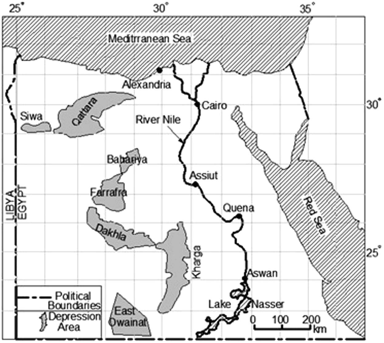
Egypt map showing the major oasis in the New Valley Governorate [4]

Groundwater exists in the fringes of the Nile Valley, Nile Delta, Western Desert and Sinai Peninsula. Groundwater aquifers which are located in Nile Valley, Nile Delta and Sinai Peninsula replenished from the river Nile by seepage from canals and deep percolation from irrigation application [5]. Groundwater in the Western Desert is the only available resource for interdisciplinary development in the desert area, and it is a non-renewable water resource [4, 6]. Developing strategies of the desert area depend on pumping costs of fossil water and potential economic return over a fixed time period. For coastal zones, groundwater reservoirs are recharged from local rainfall [7]. The largest groundwater deposit is located underneath the eastern part of the African Sahara and is shared between Egypt, Sudan, Libya and Chad as shown in Fig. 2 [8, 9].

../images/437178_1_En_84_Chapter/437178_1_En_84_Fig2_HTML.png — Fig. 2
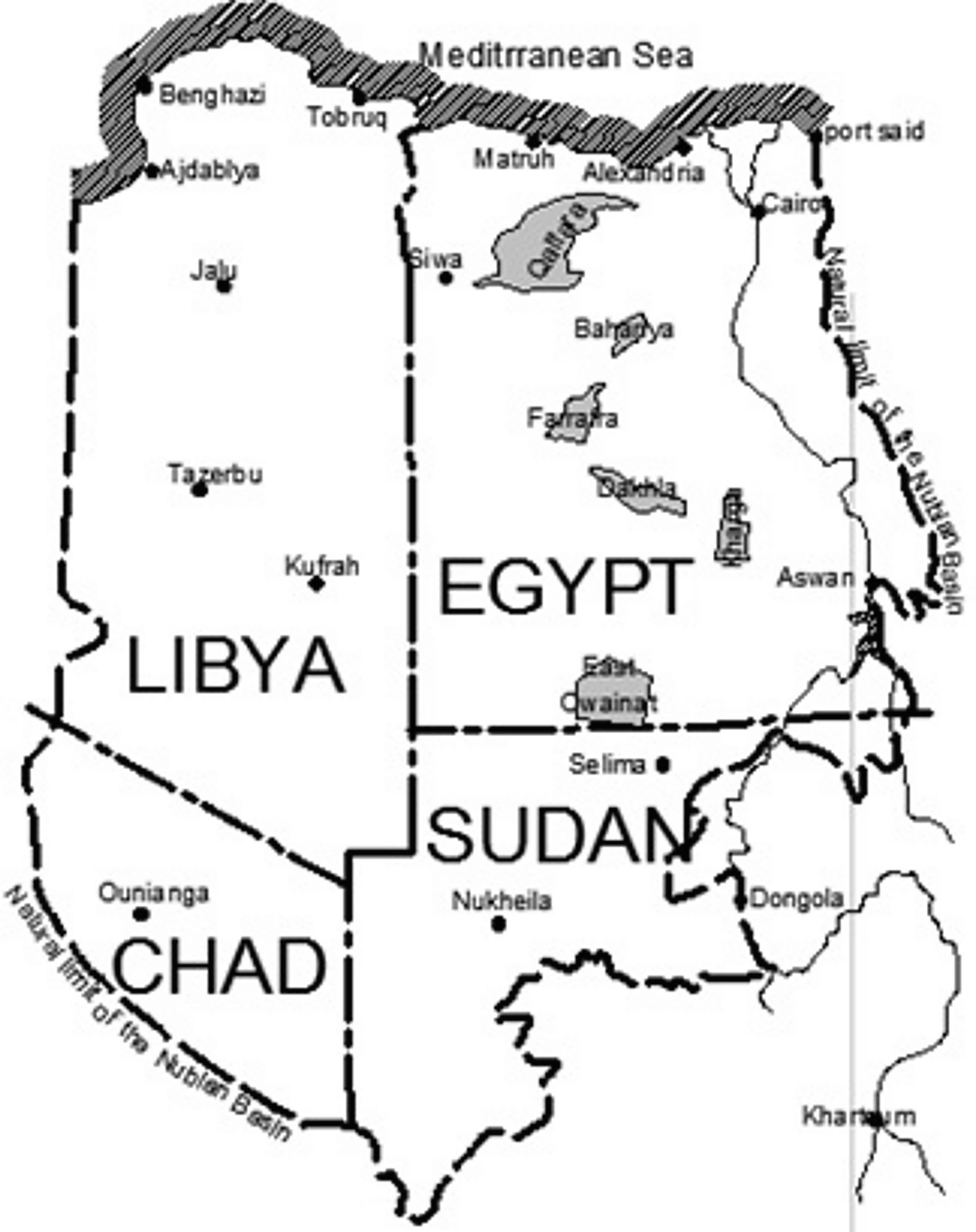
Schematic distribution of Nubian Sandstone under Egypt, Libya, Sudan and Chad [9]

2 Hydrogeology of Aquifer Systems in Egypt

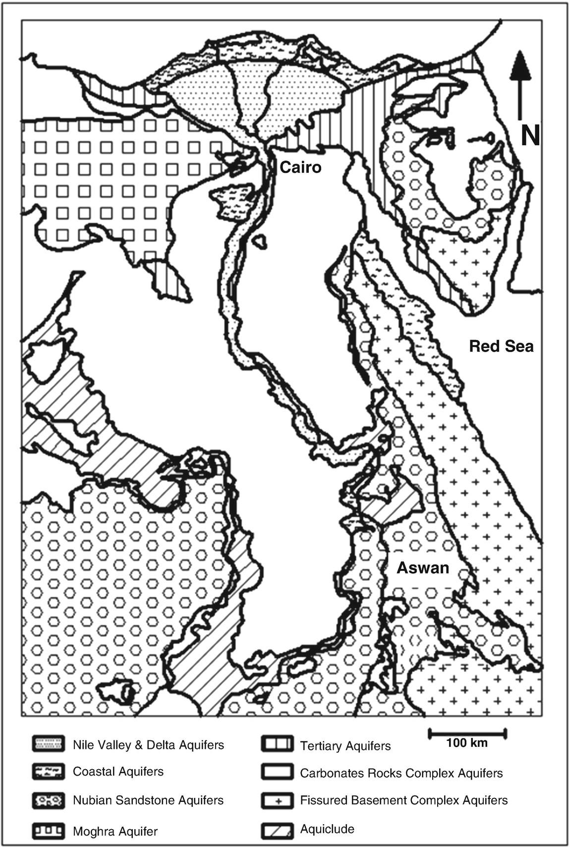
The hydrogeological framework of Egypt comprises seven aquifer systems [1, 2, 5, 7, 10–12], as shown in Fig. 3:

../images/437178_1_En_84_Chapter/437178_1_En_84_Fig3_HTML.png — Fig. 3
Hydrogeological map of Egypt [1]

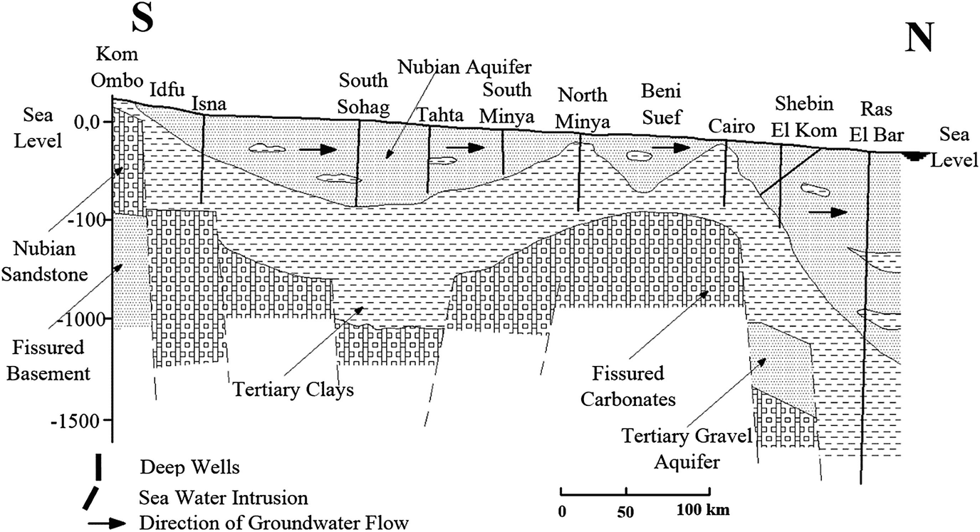
2.1 The Nile Valley Aquifer Systems (NVAS)

The aquifer assigned to the Quaternary and Late Tertiary is located under the Nile flood plain and desert fringes and consists of a thick layer of graded sand and gravel covered by a clay layer in its major part. NVAS thickness varies from 300 m in Middle Egypt (Sohag Governorate) and decreases to only a few metres to the north towards Cairo and in the south direction up to Aswan as shown in Fig. 4. Below this aquifer, there are clayey deposits that were formed during the Pliocene, which are impermeable and prevent the connection between this aquifer and the Nubian Sandstone aquifer. However, there could be a connection between the Quaternary deposits and the surrounding limestone. The water is mainly used for domestic purposes and irrigation; its salinity is less than 1,500 ppm. The aquifer system is renewable, and the main recharge source is the infiltration from the excess water application for agriculture and seepage from the irrigation water distribution system [1]. The saturated thickness of NVAS aquifer is in the range of 10–200 m. On the other hand, its hydraulic conductivity ranges from 50 to 70 m/day.

../images/437178_1_En_84_Chapter/437178_1_En_84_Fig4_HTML.png — Fig. 4
Hydrogeological profile through the Nile Valley and Delta basins [6, 13]

2.2 The Nile Delta Aquifer Systems (NDAS)

Four regional aquifers are present in the NDAS in addition to six subregional and local aquifers [1] as shown in Fig. 5. Tahlawi et al. [1] mentioned that the NDAS assigned to the Pleistocene age consists mainly of graded sand and gravel. However, to the north, it consists of fine sand and clay. NDAS is considered as semi-confined aquifer. It is overlain by Holocene silt, clay and fine sand in the floodplain of the Nile. A calcareous loamy layer acts as a semi-confining zone outside the floodplain in the north-western part of the Delta with a thickness ranging between 0 and 20 m. However, to the west, there is a hydraulic connection between the Quaternary aquifer with the Moghra aquifer. This connection could be declared by the westward continuity of the piezometric gradient (Fig. 6). In the desert fringes, the semi-confined layer is missing, and phreatic conditions prevail [1]. The thickness of the layers holding the groundwater is different from one place to another; however, its average thickness is 190 m, increasing gradually to the north until it reaches 350 m at Tanta City. At the western part of the Delta, the thickness of the layer holding water varies between 120 and 220 m, decreasing gradually towards the east. The total thickness of the aquifer increases from Cairo northward to about 1,000 m along the Mediterranean coast [7, 12]. The depth to the groundwater level in the Nile Delta aquifer increases from the north towards the south. It varies between 1 and 2 m at the north, increases to vary from 3 to 4 m at the middle and reaches maximum value 5 m at the south [14]. The Nile Valley and Nile Delta aquifer are expected to be separated as the aquifer thickness is reduced to a few metres at Cairo. The quality and quantity of the southern part of the aquifer are much better than the northern part as TDS does not exceed 1,000 ppm. The aquifer is continuously recharged by infiltration of irrigation water [1, 7]. The permeability ranges between 35 and 75 m/day, and it decreases near the coastline due to increase in clay content. The horizontal hydraulic conductivity in the Quaternary Nile Delta aquifer ranges between 0.05 and 0.5 m/day. The storage coefficient range is in the range of 10⁻⁴ to 10⁻³, while 0.3 represents the porosity of the aquifer medium. The transmissivity ranges between less than 500 m²/day at the edges in the desert fringe to more than 25,000 m²/day in the apex of the Nile Delta. The characteristics of the northern portion of that system are considerably different. The aquifer becomes less productive, containing mainly brackish or saline water due to seawater intrusion.

../images/437178_1_En_84_Chapter/437178_1_En_84_Fig5_HTML.png — Fig. 5
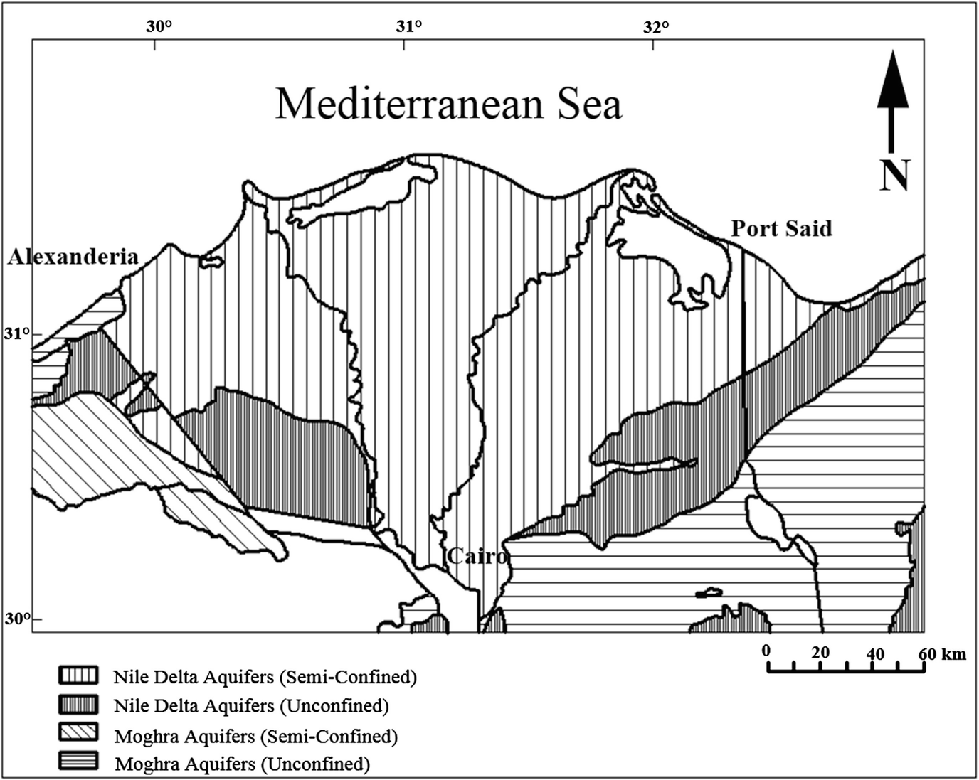
Groundwater aquifers in the Nile Delta [1]

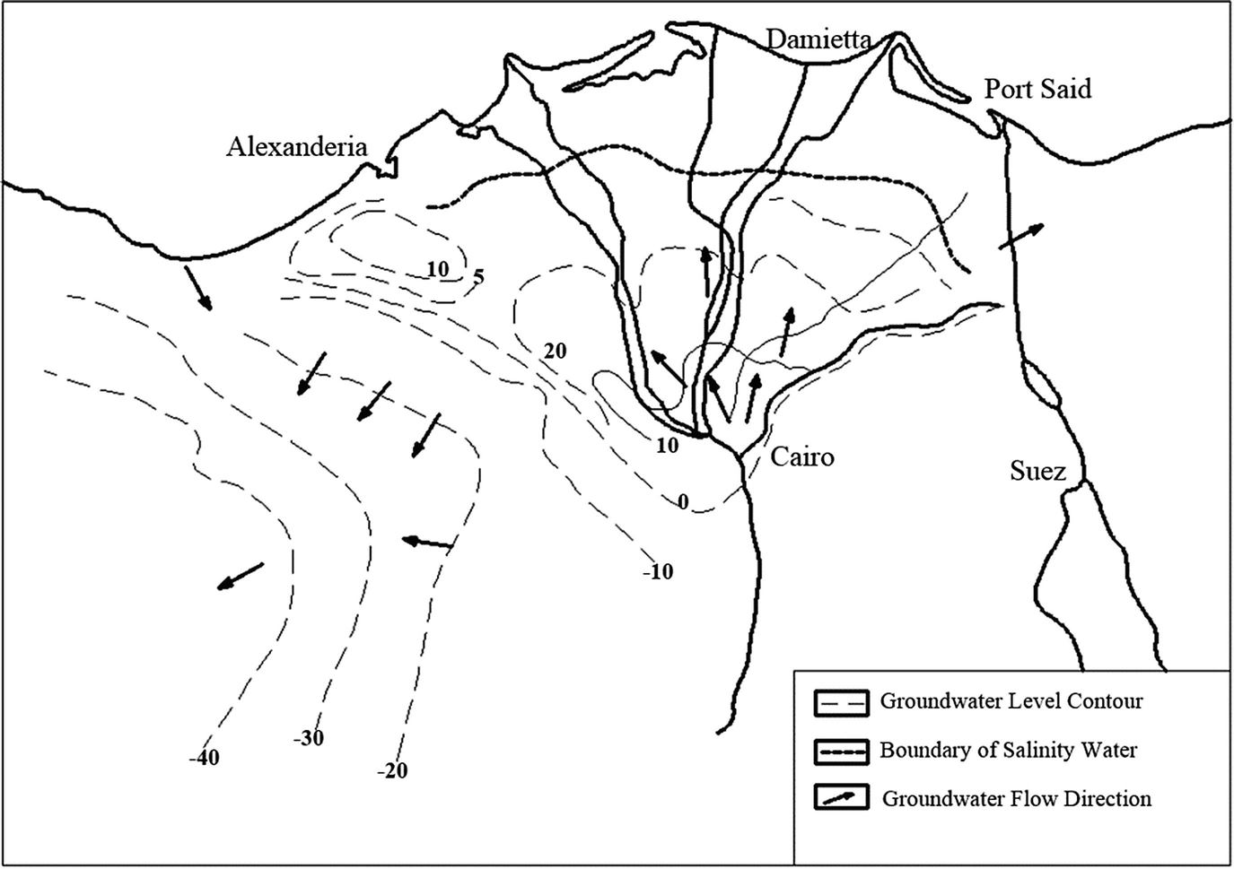
../images/437178_1_En_84_Chapter/437178_1_En_84_Fig6_HTML.png — Fig. 6
Regional groundwater levels and trends in the Nile Delta and its fringes from hydrogeological map of Egypt [1]

2.3 The Coastal Aquifer Systems (CAS)

The aquifer belongs to the Quaternary and Late Tertiary types. The systems are found along the Mediterranean and Red Sea coasts. The CAS is in the form of scattered pockets. Groundwater in CAS aquifer is in the form of thin lenses over the saline water. The aquifer is considered as renewable aquifer, and it is recharged from rainfall [9].

The CAS aquifer could be divided into two zones, the Mediterranean and Red Sea littoral zones. For the Mediterranean littoral zone, it occupied an area about 10,000 km². It is characterized by relatively high rainfall up to 200 mm/year. On the other hand, many local aquifer systems are located in the Mediterranean littoral zone. These aquifers are represented by the oolitic limestone aquifer dominating the area to the west of the Nile Delta and by the complex fluviatile sandy gravels and the shallow marine calcareous limestone in North Sinai, near El Arish. On the west of the Nile Delta, the oolitic limestone aquifer has a thickness of 40 m. The aquifer is recharged from winter rainfall and exists under phreatic conditions. It forms a thin layer (±1.0 m thick) floating on the saline water body resulting from seawater intrusion [1].

At El Arish in northern Sinai, the aquifer is characterized by a top sandy aquifer, a middle fluviatile gravelly aquifer and a lower calcareous sandstone aquifer. For the first, it is known as Thaimail, and the groundwater is recharged by local rainfall and occurs at shallow depth from the surface (±2.0). For the middle fluviatile gravelly aquifer, its thickness is about 30 m; the groundwater there is under semi-confined conditions and found at a depth of about 15 m from the surface and is capped by a clayey layer. The last aquifer is the lower calcareous sandstone aquifer which is known also as Kurkar. It is of shallow marine origin and has a wide geographical distribution in northeastern Sinai. It has a thickness of 40 m and extends inland for a distance of about 15 km from the coast. This aquifer directly underlies the fluviatile gravelly aquifer and is connected hydrologically. It is recharged in the foot slope area of Sinai highland, by local rainfall, by runoff water and presumably also by the upward leakage from the high pressure water in the Nubian Sandstone Aquifer System underlying the area. The salinity of the water varies between 3,000 and 5,000 ppm.

For the Red Sea coast aquifers, it extends also into Sinai, comprising essentially the quaternary fluviatile aquifer and the tertiary aquifers. The groundwater in the quaternary fluviatile aquifer is under phreatic conditions with a hydraulic head level same as sea level. For the tertiary aquifers, they are recharged by runoff water, by infiltration from the quaternary aquifers and locally by upward leakage from deep-seated aquifers. The salinity is about 2,000–2,500 ppm.

2.4 The Nubian Sandstone Aquifer System (NSAS)

The NSAS is a regional system and considered as a non-renewable aquifer system. It extends into Libya, Sudan and Chad and western Saudi Arabia with a total area of about two million kilometres. The groundwater volume of NSAS is about 150,000 km³ [15]. NSAS in Egypt could be divided into five subsystems with respect of their locations: at the Western Desert, at Nile Valley, at the Eastern Desert, at Gulf of Swiz and at Sinai. For the NSAS at the Western Desert, it is exploited particularly in the New Valley area, where intensive deep drilling was carried out during the past five decades. There are more than 500 wells that have been drilled to depths from 500 to 1,000 m. Groundwater flow in this aquifer (under New Valley) is towards the northeast with a gradient of 0.5 m/km. The hydraulic parameters are determined in various parts of the New Valley: Kharga, Dakhla, El Bahariya (El Bauity), El Farafra and southward east of Oweinat area. At Kharga and Dakhla Oasis, the salinity decreases from 600 in the upper layers to 200 ppm in the lower layers. On the other hand, NSAS at the Nile Valley extends from the north to the south up to Aswan. West of Cairo, groundwater has been found at a depth of 1 km with high salinity. However, the hydrogeological information about this aquifer is insufficient. The springs of Helwan are mainly connected to this aquifer. At Eastern Desert, NSAS appears in many zones such as El Laqeita area and east of Qena. At El Laqeita area, the groundwater is flowing freely, and the piezometric level is up to 112 m above mean sea level (MSL). The salinity varies in the Eastern Desert between 1,000 and 10,000 ppm. For the NSAS that lies under Gulf of Swiz, its water originates from the watershed in Sinai with salinity about 100,000 ppm. In Sinai Peninsula, NSAS water is basically a fossil water (Late Pleistocene). It is recharged from the uptake areas in Southern Sinai, where the rainfall rate is about 120 mm/year. The flow pattern is in the northward direction. Sinai is bounded by two major rift valley basins, and the local groundwater flow direction is towards these basins: westward in Western Sinai and eastward in the East. Consequently, springs are present near the Gulfs of Suez and Aqaba. In Central Sinai, the piezometric level is about 200 m above sea level, and at the springs of Oyun Moussa (south of Suez), it is close to sea level. The salinity of the water in Central and Southern Sinai is of the order of 1,500 ppm, but it increases to more than 5,000 ppm in North and West Sinai.

2.5 The Moghra Aquifer System (MAS)

The aquifer assigned to the Lower Miocene occupies mainly the western edge of the Delta up to the Qattara Depression. The MAS outcrops on the surface in Wadi El Natrun and Wadi El Farigh [1, 6] illustrate that MAS aquifer has an average thickness of 300 m and is considered as a non-renewable aquifer system. The hydraulic gradients have a value less than 0.2 m/km. The groundwater in the MAS aquifer is a mixture of fossil and renewable water. Discharge of the aquifer is through evaporation in the Qattara and Wadi El Natrun depressions and through the lateral seepage into carbonate rocks in the western part of the Qattara Depression. The base of the aquifer slopes from ground level near Cairo to 1,000 m below mean sea level west of Alexandria. The saturated thickness is between 70 and 700 m. Permeability ranges between 25 m/day east of Wadi El Farigh to less than 1 m/day in the Qattara area and near the coast. Transmissivity ranges between 500 and 5,000 m/day. The salinity of the water changes from less than 1,000 ppm in the east, i.e. close to the main recharging area, to more than 5,000 ppm in the west, i.e. close to the main discharging area.

2.6 The Karstified Carbonate Aquifer System (KCAS)

KCAS is assigned to the Eocene and to the Upper Cretaceous. It predominates essentially in the north and middle parts of the Western Desert. Although the fissured and karstified carbonate aquifer complex occupies at least 50% of the total area of the country, it is the least explored and exploited in Egypt. The recharge to this aquifer is essentially from the upward leakage from the underlying Nubian Sandstone aquifer, and El Tahlawi et al. [1] mentioned that the carbonate complex is generally divided into three horizons: lower horizon assigned to Upper Cretaceous, middle horizon assigned to Lower and Middle Eocene and upper horizon assigned to Middle Miocene. These three horizons are separated by Esna Shale (±100 m) and Daba Shale (200 m). KCAS generally overlies the Nubian Sandstone complex. The hydrogeology of the fissured limestone is not well understood. In Siwa Oasis, the fissured limestone complex has a thickness of about 650 m (Upper Cretaceous to Middle Miocene) and is lying unconformably on the Nubian Sandstone complex. Over 200 natural springs have a total flow of about 200,000 m³/day pumping out water from the top portion of the fissured limestone (Middle Miocene). Groundwater salinity there is from 1,500 to 7,000 ppm. On the other hand, test drilling in Siwa area points to the occurrence of water with a salinity of about 200 ppm in the underlying limestone, which belongs to the Eocene and the Cretaceous.

2.7 The Fissured Hard Rock Aquifer System (FHRAS)

The Fissured Hard Rock Aquifer System is mainly located in the Eastern Desert and Sinai and assigned to the Pre-Cambrian type. This aquifer is influenced by many factors including, namely, tectonic, morphotectonic and lithologic. Figure 7 shows the distribution of the outcropping and subsurface basement rocks.

../images/437178_1_En_84_Chapter/437178_1_En_84_Fig7_HTML.png — Fig. 7
Distribution of basement rocks in Egypt [1, 16]

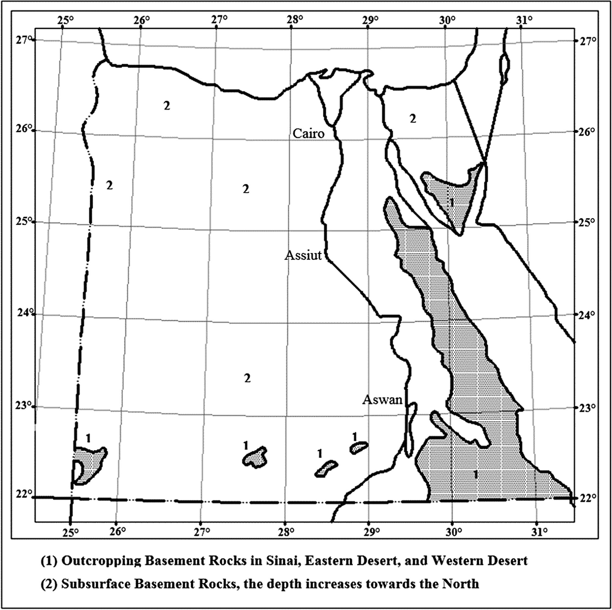
3 Nubian Sandstone Aquifer System in Western Desert

The aquifer assigned to the Paleozoic–Mesozoic occupies a large area in the Western Desert and parts of the Eastern Desert and Sinai. Groundwater can be found at very shallow depths, where the water-bearing horizon is exposed, or at very large depths (up to 1,500), where the aquifer is semi-confined. The NSAS is a regional system. It extends into Libya, Sudan and Chad, and it is a non-renewable aquifer system Mahmod et al. [4], Mahmod and Watanabe [6], Ebraheem et al. [17] illustrate that the Nubian Sandstone Aquifer System (NSAS) is considered to be the largest fossil groundwater aquifer system in the world and is located under the eastern end of the Sahara Desert. NSAS groundwater is shared among Egypt, Libya, Sudan and Chad (see Fig. 2). In Egypt, the NSAS extends under the New Valley Governorate area, where it acts as a local major water source. The total area of the aquifer is approximately 630,000 km² and at some areas reaches to a depth of 3.5 km below the ground surface [18]. The recharge of the NSAS aquifer is thought to be generally negligible [19]. Due to overuse of NSAS groundwater for industrial and agricultural applications during the last two decades, a significant drawdown in the groundwater table has been observed. The origin of groundwater in the NSAS has been extensively discussed by several authors since approximately 1920; two possibilities for the origin have been proposed. The older postulated concept is that the groundwater is supplied from precipitation in the southern mountainous parts of the NSAS. This concept was suggested primarily by Ball [20] and supported by Sanford [21]. The newer postulate by Sonntag [22] suggested that the bulk of the groundwater mass within the aquifer was originally supplied in situ during the humid pluvial periods (up to 30,000 years B.P.). There are three possible ways of groundwater recharge: regional groundwater influx from areas with modern groundwater recharge, local infiltration through precipitation during wet periods in the past and finally post-High Dam construction seepage of Nile water [24]. In addition, [20, 21, 23] noted that the general flow direction in the NSAS is from the southwest to the northeast Thorweihe and Heinl [25] found that the amount of the current recharge to the NSAS from the south is not significant based on the groundwater velocity, aquifer resistance time and climatic conditions.

The geology of the Western Desert of Egypt, including the Kharga Oasis, has been well documented by many geologists [21, 26–28]. The NSAS is a confined aquifer that is overlaying an impermeable crystalline rock that comprises the lower confining layer. The upper confining layer is an impermeable variegated shale and clay overlying the Nubian Sandstone aquifer. The NSAS is composed of a series of mostly unfossiliferous formations. In the Kharga Oasis as an example, NSAS formations are comprised of sands, sandstones, clays and shales (see Fig. 8). The NSAS formation changes gradually from primarily continental sandy facies in the southern region (Sudan) to intercalations of sandstones and clays of alternating continental and shallow marine facies in the central region (e.g. the Kharga Oasis). The formation then changes to marine facies in the northern region (Qattara Depression), where it consists of thick beds of clays intercalated with beds of limestone, dolomites and sandstones. It is generally thought that the geological age of the NSAS ranges from the Cambrian to the Upper Cretaceous period [29].

../images/437178_1_En_84_Chapter/437178_1_En_84_Fig8_HTML.png — Fig. 8
Lithostratigraphic sections across the study area [4, 6, 9]

Lamoreaux et al. [23] and Thorweihe and Schandelmeier [30] reported that the thickness of the Nubian Sandstone aquifer beneath the Kharga Oasis ranged from 300 to 1,000 m. Shata [31] noted that in the Kharga Oasis, 32 water-bearing horizons had been recognized within the Nubian Sandstone succession. Shata [31] grouped these water-bearing horizons into three aquifers that include (1) a top layer with an average thickness of 200 m, (2) a middle layer with an average thickness of 200 m and (3) a lower layer with a thickness of approximately 250 m. Lamoreaux et al. [23] mentioned that the NSAS consists of thick sequences of coarse, clastic sediments of sandstone and sandy clay interbedded with shale and clay beds. These clayey impermeable beds restrict the vertical movement of water among water-bearing layers. These beds of lower permeability, however, are lenticular and discontinuous; thus, regionally, the Nubian sandstone forms a single aquifer complex.

4 Groundwater Modelling and Uncertainty

4.1 Model Types

A model is a simulation of areal and temporal properties of a system, or one of its parts, in either a physical or mathematical way. The difficulties of building physical model are obvious in how feasible is the water table (hydraulic head) in a multilayer aquifer exposed to various stresses such as precipitation, surface runoff and leakage from deep underlying strata and then change some of its geometric and hydrogeological properties as needed. For these difficulties, the application of real physical models has been limited to educational and demonstration purposes. Mathematical models are those equations used to analyse groundwater flow. Three mathematical models could be identified; depending upon the nature of equations involved, these models can be empirical, probabilistic and deterministic models. Empirical models are derived from experimental procedures until relations are fitted to some mathematical function. Although empirical models are limited in scope, they can be an important part of more complex problems. Probabilistic (stochastic) models are based on statistics such as probability. These models either have various simple probability distributions of a hydrogeological information or complicated stochastic, time-dependent models. The main problem of the stochastic models, for a wider use in hydrogeology, is that they need large data sets for parameter identification. Moreover, it is difficult to predict the future behaviour of groundwater flow under any change of water table stress. Deterministic models are those models that are predetermined by physical laws governing groundwater flow such as Theis equation and Darcy’s law. These types of models are used to solve complicated groundwater problems as a multiphase flow through a multilayered, heterogeneous, anisotropic aquifer system. There are two categories of deterministic models: analytical and numerical models. Analytical models are used to solve one equation of groundwater flow at a certain time for one point or line of points. Analytical models are easy to be applied to one point with homogeneous aquifer property. Calculation time is increased if the model is applied for many points and if the aquifer is quite heterogeneous. If the situation gets really complicated, such as when there are several boundaries, more pumping wells and several hydraulically connected aquifers, the feasible application of analytical models terminates. Numeric models describe groundwater flow for many points as specified by the user considering heterogeneity of the aquifer. This is achieved by dividing the area of interest into small subdivisions named cells or elements. Then, a basic groundwater flow equation is solved for each cell considering its water balance. The outputs are a distribution of hydraulic heads at points representing individual cells. These points can be placed at the centre of the cell, at intersections between adjacent cells or elsewhere. These models are coded by solving the basic differential flow equation for each cell approximately to finally get an algebraic equation that can be easily solved through an iterative process (numeric) solution. The two most widely applied numeric models are the finite difference model (FDM) and finite element model (FEM). The difference between FDM and FEM is mainly at approximation of the differential flow equation until getting the algebraic equation to be solved then by iterative process.

4.2 Source of Uncertainty

Groundwater management in many arid areas in the world has been difficult due to the limited availability of hydrogeological data. The lack of basic data often limits the implementation of the numerical models for groundwater flow analysis, as well as introduces a problem for model calibration and validation. A deterministic approach is useful to overcome the uncertainty because it depends on variables or parameters with values determined by taking into account previously collected historical information. Although this type of approach has some limitations, it can be very useful in the decision-making process. It is relatively simple and allows for a detailed exploration of other aspects that are sometimes neglected in more sophisticated models.

There are many sources of uncertainty in groundwater analysis. The most common sources are:

Natural variability of hydrologic properties of the groundwater aquifer
Limited and incorrect information on hydrogeological variables and parameters that characterize the groundwater flow
Lack of information on future groundwater exploitation rate because of temporal changes of anthropogenic activities, land use, land cover, and climate change

Sensitivity analysis is a straightforward technique that allows the identification of the parameters and variables that have more influence on system performance and allows evaluation of the scale of this influence. Uncertainty in constraints can also be modelled using several different techniques. When uncertainty is small, it can be done in terms of expected values. Chance-constrained models are very useful in reliability analysis (reliability expresses the probability of a system operating without failure). Chance-constrained models describe constraints in mathematical models in the form of probability levels of attainment. The chance constraints can be converted into deterministic equivalents and can therefore be easily incorporated into deterministic programming models. From the previous two sections, it could be concluded that it is difficult to develop a proper groundwater management system given such uncertainties and data limitations when using ordinary numerical models.

5 Overcoming Uncertainty

To implement an optimal groundwater management, temporal and spatial variation of groundwater table should be investigated first as an indispensable factor in groundwater flow analysis. Temporal and spatial variation of groundwater table is an important factor for implementing the optimal management of groundwater resources. A model is suggested to make clear this spatial distribution of groundwater flow by analysing spatial relationships among OWs considering the limited availability of data. This model is linear regression model. Genetic algorithm (GA) was adapted as a technique to estimate the optimized values of the linear parameters considering robustness and high conversion of this method as one of the soft computing techniques (SCTs). This mentioned technique quantifies the spatial structure of the data and produces a prediction of pore pressure change at arbitrary points. A newly developed model named the grey model (GM) was adopted to analyse groundwater flow. This model combines a finite element method (FEM) with GA model to try to obtain the best-fit piezometric level trends compared to observations. On the other hand, the GM has no clear theories that exist for selecting the number of input model trends and the most suitable values of input parameters. Therefore, a modification of the GM is newly proposed and called the modified grey model (MGM) in an attempt to determine a process for selecting the best input models’ trends with the appropriate values of input parameters to achieve acceptable fitting to observations.

5.1 Grey Model (GM)

GM is a combination of a 2D-FEM with genetic algorithms (GA) as the NM and SCT, respectively. FEM was used to analyse groundwater flow under the assumption of hydrogeological and boundary conditions to produce approximate solutions for temporal piezometric level changes. The GA model was used to fit the measured temporal piezometric level changes.

Although the GM has been proposed by some hydrogeologists, it has not yet been widely applied to groundwater problems. The main concept of the GM is combining a numerical model (NM) with a soft computing technique (SCT) Mohammed et al. [32] proposed a GM as a combination of a 3D-FEM with an artificial neural network (ANN) as the NM and SCT, respectively Mohammed et al. [32] used a GM to predict the piezometric level change in the fractured rock mass at Mizunami Underground Research Laboratory (MIU), Japan. In the current study, an FEM and a linear regression model based on genetic algorithms (GAs) were used. FEM was used to analyse groundwater flow under the assumption of hydrogeological and boundary conditions to produce approximate solutions for temporal piezometric level changes. The GA model was used to fit the measured temporal piezometric level changes.

5.1.1 Model Structure

Due to the uncertainty in the hydraulic parameters for water-bearing layers and lack of information about the pumping rates from each layer, it was difficult to properly construct a 3D-FEM model. In addition, the OWs do not provide piezometric level data for specific aquifer layers but rather for the entire deep aquifer (layers B, C and D). Because of these considerations, a 2D-FEM was applied in this study. The governing equation for saturated groundwater flow can be obtained by combining a special form of Darcy’s law (derived from the water phase momentum balance) and the continuity equation written for the water phase [33, 34], as given in the equation

$\frac{\partial }{\partial x}\left({T}_{xx}\left(\frac{\partial h}{\partial x}\right)\right)+\frac{\partial }{\partial y}\left({T}_{yy}\left(\frac{\partial h}{\partial y}\right)\right)=S\left(\frac{\partial h}{\partial t}\right)-W$

where T _xx and T _yy are the transmissivities along the x and y directions, respectively, h is the hydraulic head, S is the storativity, W is the groundwater volume flux per unit area (positive for outflow and negative for inflow), x and y are the Cartesian coordinates and t is the time.

The FEM calculations were carried out assuming n different 2D hydrogeological models. For each model, the grid geometry and number of elements were identical. However, different sets of hydrogeological conditions, such as horizontal transmissivity in the x and y directions (T _xx and T _yy) and specific storage and boundary conditions were assumed for each model. Then, n piezometric level trends (H ₁(t), H ₂(t),…,H _n(t)) were calculated by FEM. These simulated piezometric level trends were not representative of the measured piezometric level trends. The linear model was used to reconstruct the measured piezometric level trend by combining FEM output piezometric level trends (H ₁(t), H ₂(t),…, H _n(t)) as given in the equation

${H}_s(t)=\sum \limits_{i=1}^{i=n}{\alpha}_i\cdot {H}_i(t),\kern0.5em \sum \alpha =1$

where H _s(t) is the reconstructed piezometric level trend at a certain location, H _i(t) are the 2D-FEM simulated piezometric level trends, and α _i are weight parameters for the linear regression model. The best-fitting parameters for the linear model are estimated by a GA model. The weight parameters can also be used for future prediction of temporal piezometric level change at any time (t). The structure of the GM is schematically illustrated in Fig. 9.

../images/437178_1_En_84_Chapter/437178_1_En_84_Fig9_HTML.png — Fig. 9
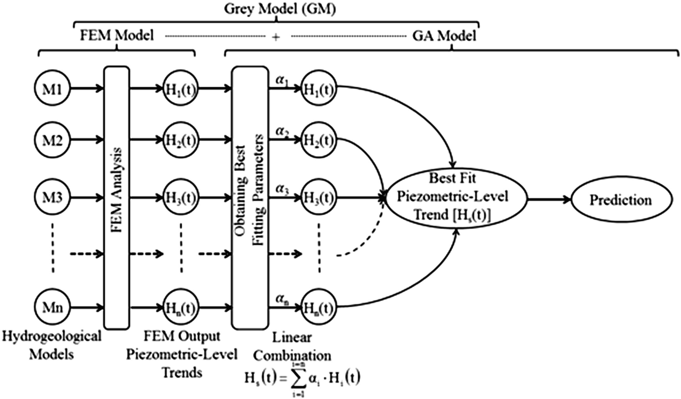
Structure of the developed grey model [4]

The basic process of the GA used in this study is as follows (see Fig. 10):

1.
Generate N different chromosomes by giving random values in the range of 0.0–1.0 as genes. The gene values are adjusted to fit the criterion that the sum of the genes in each chromosome should equal 1.0. The number of chromosomes N is called the population size, and all chromosomes are put in the initial (1st) pool representing the first generation.
2.
The previous equation is applied to obtain the reconstructed piezometric level trend (H _s(t)). Then, the root mean square error (RMSE) and fitness value (F _i) between the measured (H _o(t)) and the reconstructed piezometric level trends (H _s(t)) for every chromosome are calculated. Chromosomes in the first pool are rearranged based on the probability value of each chromosome (rating process):

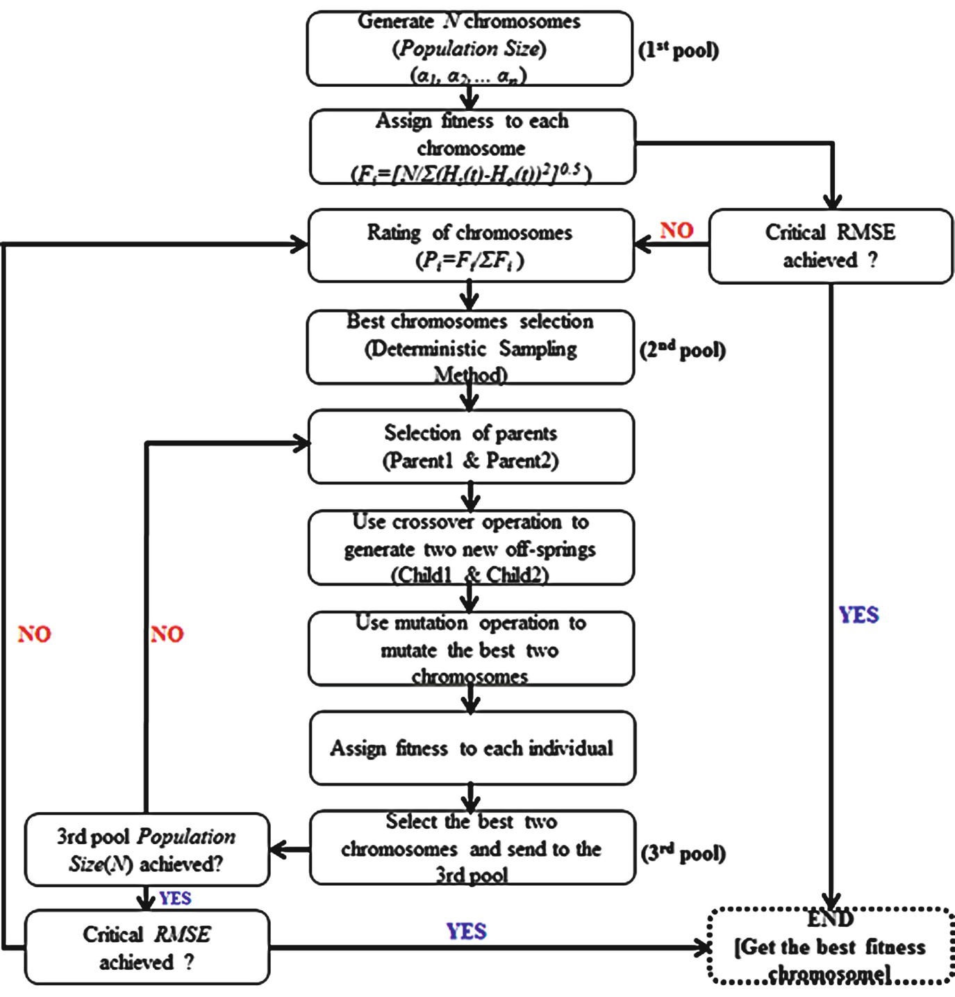
../images/437178_1_En_84_Chapter/437178_1_En_84_Fig10_HTML.png — Fig. 10
Flow chart describing the GA optimization process [4]

${F}_i=\sqrt{\frac{N}{\sum \limits_{i=1}^{i=N}{\left({H}_S(t)-{H}_o(t)\right)}^2}}=\frac{1}{\mathrm{RMSE}}$

${P}_i=\frac{F_i}{\sum \limits_{i=1}^{i=N}{F}_i}$

3.
Based on the rating process, the best-fit chromosomes are selected and sent to fill the 2nd pool. The selection of chromosomes was performed by using a deterministic sampling method [35, 36]. In this method, the average fit of the population is calculated. Then, the fitness for each chromosome is divided by the average fitness, but only the integer part of this operation is used to select individuals to send to 2nd pool. The entire fraction is used to sort the individuals. The remaining free places in the new population are filled with the chromosomes that have the largest fraction values in the sorted list.
4.
Two chromosomes are selected randomly from the second pool and are called parent chromosomes. Two offsprings are created from the parents by using a crossover operation. A crossover is a process to mix the genes of parent chromosomes. In this study, a two-point crossover technique was used [37, 38]. By using the chromosomes of parents and children, four temporal piezometric level trends are calculated, and then two of these trends with a large value of F _i are selected. The ratio between the number of chromosomes thus created and the population size is called the crossover probability.
5.
The selected two chromosomes constructed and calculated by the crossover process were mutated by changing some gene values using random numbers between 0.0 and 1.0. After mutation, the sum of the gene values should equal 1.0. Among the four chromosomes, the two chromosomes that have the best-fitting values are sent to the 3rd pool. The ratio between the mutated gene and all genes of one chromosome is called the Mutation Probability. Crossover and mutation are repeated until the population size of the 3rd pool is filled; this process is referred to as the second generation.
6.
The process from step 2 to step 5 is repeated for a fixed number of generations or until the error between measured and calculated piezometric level trends falls below an assumed critical RMSE value.

All steps from 1 to 6 are applied to a portion of the time series data to train the model (training/learning phase). The other part of the data is used for validation of the resulting weights (prediction/test phase). Due to the limitation of data and to guarantee good results in the prediction phase and future assessments, the majority of the data series is used in training, while the rest is left for the prediction phase.

5.2 Modified Grey Model (MGM)

In the GM, the used GA model has no clear concept for selecting the number of input piezometric level trends and values of input parameters. The input piezometric level trends are the calculated piezometric level trends from the assumed hydrogeological models. On the other hand, the input parameters are the parameters which used to fit the measured observations such as population size, crossover probability, mutation probability and number of generations. For simplicity, in the current study, the number of input piezometric level trends will be named as input models’ trends.

In the current study, this concept is processed, and new model named as modified genetic algorithm (MGA) is proposed trying to select the best input models’ trends for fitting to the measured piezometric level trends. Moreover, the effect of number of input models’ trends on the values of input parameters was studied by meaning of sensitivity analysis for both models GA and MGA. By combining this new proposed model MGA with the FEM model, a new model is produced and named as modified grey model (MGM).

In the current study, the MGM was newly developed for the analysis of groundwater flow. Broadly speaking, the main concept of the MGM is quite similar to the GM because it combines a numerical model (NM) with a soft computing technique (SCT). The GM has not yet been widely applied to groundwater problems. In the GM, the number of input models’ trends and the values of the input parameters are selected hypothetically before obtaining the best-fitting values [4, 32]. The main problem in the GM is that there is no clear concept in the GA model for the selection of either the number of input models’ trends or the values of input parameters, such as population size, crossover probability, mutation probability and number of generations (fitting calculation time). For this purpose, a modification of the GA model was developed to select the input models’ trends that achieve the best fit to the observations. Then, the effects of the best selected models’ trends on the values of GA input parameters were studied. The GA model after modification will be called the modified genetic algorithm (MGA) model. The combination of the best models’ trends will be called the best models combination (BMCk, where k is the number of selected models’ trends). The MGM is the combination of FEM and MGA. As an application for MGM, this model is used to evaluate three different future exploitation/development plans under consideration for the aquifer system to explore the hydrological feasibility of these plans. The MGM simulation is applied for the period from the year 1960 to the year 2100.

5.2.1 Model Structure

The FEM calculations were carried out assuming n different 2D hydrogeological models. Then, n piezometric level trends (H ₁(t), H ₂(t),…,H _n(t)) were calculated by FEM. These simulated piezometric level trends were not representative of the measured piezometric level trends. The linear model (GA model) was used to reconstruct the measured piezometric level trend by combining the calculated piezometric level trends (H ₁(t), H ₂(t),…,H _n(t)), as given in the equation below. For MGA, only the best models’ trends were selected to be combined together by the best model combinations (BMC_k (R ₁(t), R ₂(t),…R _k(t), where R _k is the selected models’ trends from H _n models’ trends) to match the target measured trend:

${R}_s(t)=\sum \limits_{j=1}^k{\alpha}_j\cdot {R}_j(t),\kern0.5em \sum {\alpha}_j=1,{\displaystyle \begin{array}{cc}& \end{array}}k\le n$

where R _s(t) are the reconstructed piezometric level trends at a certain location estimated by MGM; R _j(t) is the 2D-FEM simulated piezometric level trends; and α _j are weight parameters. The produced weight parameters can also be used for the future prediction of temporal piezometric level changes at any time (t). The structure of the MGM is schematically illustrated in Fig. 11.

../images/437178_1_En_84_Chapter/437178_1_En_84_Fig11_HTML.png — Fig. 11
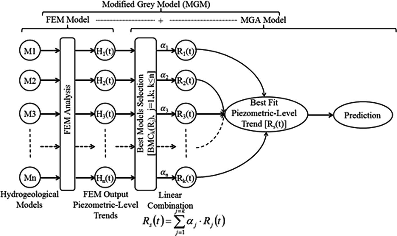
Structure of the developed grey model [6]

Many researchers reported that the GA model provides good performance for estimating the optimum combination of weight parameters [4]. This combination of weight parameters is called a chromosome (α ₁, α ₂,.. α _n), and each weight parameter is called a gene. However, the optimum number of inputs (hydrogeological models) and the values of the input parameters remain a problem. For this reason, the GA model has been modified by adding a selection process for finding the optimum input models’ trends. This newly developed model is called the modified genetic algorithm (MGA) model. The selection process is used for selecting the best inputs that achieve an appropriate goodness of fit with the measured piezometric level trends. The number of selected inputs is “k,” and the combination of these inputs is called the best models combination (BMC_k). The concept of the proposed model (MGA) could be described in two stages, as follows (see Fig. 12) [4, 39]:

../images/437178_1_En_84_Chapter/437178_1_En_84_Fig12_HTML.png — Fig. 12
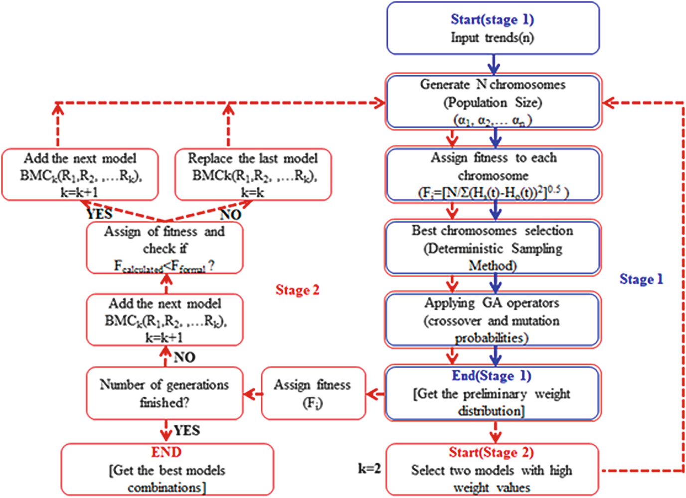
Flow chart describing the MGA optimization process [6]

Stage 1 (Preliminary weight distribution): The process in this stage is the same as in the ordinary GA model [4]; however, the target of this stage is not determining the optimum weight parameters. This stage is used to obtain a preliminary weight distribution for the inputs with any value for number of generations. For this reason, using a small number of generations is enough to obtain this type of distribution. This stage contains the following main steps:

1.
After simulating groundwater flow using the hydrogeological model explained previously, n temporal trends of hydraulic heads (H ₁(t), H ₂(t),…,H _n(t)) are obtained and used as inputs to the GA model. Then, N different chromosomes are generated by giving random values in the range of 0.0–1.0 as genes. The gene values are adjusted to fit the criterion that the sum of the genes in each chromosome should equal 1.0. The number of chromosomes N is called the population size.
2.
As the second step of the basic process of the GA model, the reconstructed piezometric level trend (H _s(t)) is obtained. Then, the fitness values (F _i) between the measured (H _o(t)) and the reconstructed piezometric level trends (H _s(t)) for every chromosome are calculated.
3.
The best-fit chromosomes are selected using a deterministic sampling method. In this method, the average fit of the population is calculated. Then, the fitness for each chromosome is divided by the average fitness, but only the integer part of this operation is used to select individuals. Then, the entire fraction is used to sort the individuals. The remaining free places in the new population are filled with the chromosomes that have the largest fraction values in the sorted list.
4.
These “n” models’ trends are processed by GA processes (crossover and mutation processes) to obtain the final weight parameters (α ₁, α ₂,.. α _n). At the initial stage, the weight parameters are given as random numbers. Then, the weight parameters are pursued through the repetition of crossover and mutation processes until completing the selected number of generations. Crossover and mutation processes are represented by two operators: crossover probability and mutation probability.

Stage 2 (Obtaining the BMC_k(R _j(t)); j = 1,k; k ≤ n): Regarding stage 1, the weights of each input for fitting the observed trend were recognized. In this stage, the inputs are renamed according to their weights from R ₁(t) for the highest weight input to R _n(t) for the lowest weight input. Hereafter, the following steps take place:

1.
The first two inputs (BMC_k(R _j(t)); j = 1,k; k = 2) are combined using the GA model (stage 1 procedures). Then, R _s(t) is calculated, and the fitness with the observed trend R _o(t) is calculated.
2.
The third input R ₃(t) is added to the formal combination to become BMC₃(R ₁(t), R ₂(t), R ₃(t)), and then the fit is recalculated.
3.
If the calculated fit is less than the formal fit (F _calculated < F _formal), then the input will be added to the combination to become BMC₄(R ₁(t), R ₂(t), R ₃(t), R ₄(t)). On the contrary, if the calculated fit is larger than the formal fit, the last input in the combination BMC₃(R ₁(t), R ₂(t), R ₃(t)) will be replaced by its next input to become BMC₃(R ₁(t), R ₂(t), R ₄(t)). This process is continued until the selected number of generations has been completed.
4.
The best models combination (BMC_k((R ₁(t),R ₂(t),…R _k(t)) is obtained.

The two stages explained above are applied on a part of the time series data as training for the model (training phase). The other part of the data is used for the validation of the resulting weights (test phase). Due to the limited data and to guarantee good results at the prediction phase and in future assessment, a large percentage of the data is used in the training phase, and the other remains for the prediction phase.

6 Application of MGM on the NSAS Under Kharga Oasis

As applications of the new proposed model MGM, future assessment of piezometric level change was analysed by developing three exploratory scenarios of groundwater withdrawal that involved either expanding the present extraction rate or redistributing the groundwater withdrawal over the recent working production wells (RWPWs).

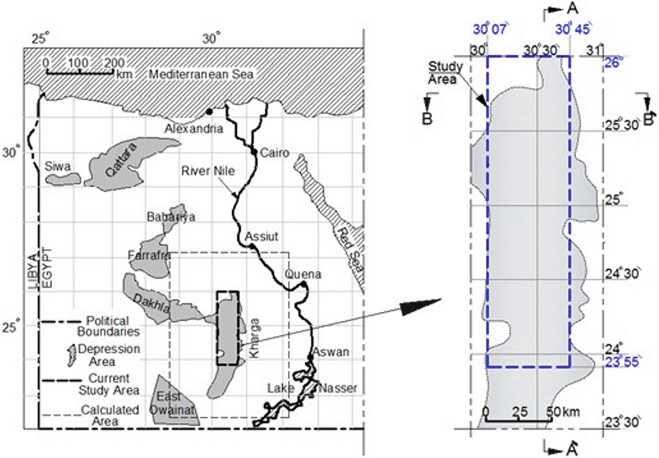
The Kharga Oasis is one of the depressions located in the New Valley in the southern part of the Western Desert of Egypt (Fig. 1). This oasis is bounded by the Eocene limestone plateau on the east and north, where steep cliffs form a sharp boundary. This limestone plateau stretches along Middle and Upper Egypt at an elevation up to 550 m above mean sea level (amsl) (approximately 400 m above the depression floor of the oasis). The studied area lies between the latitudes of 23° 55′ to 26° N and the longitudes 30° 7′ to 30° 45′ E, as shown in Fig. 13. The calculated area shown in Fig. 13 is used in the numerical analysis, as explained below.

../images/437178_1_En_84_Chapter/437178_1_En_84_Fig13_HTML.png — Fig. 13
Location map of the study area showing observed sites [6]

The Kharga Oasis is situated in the tropical arid climate zone. The maximum daytime temperature reaches up to 45–50 °C in the summer; however, the temperature drops below zero °C at night in the winter. The Kharga Oasis is one of the driest areas of the Eastern Sahara, which thus makes it one of driest areas on Earth [39]. The average potential evaporation rate reaches approximately 18.4 mm/day, and the mean annual value of the relative humidity is approximately 39%. The annual precipitation is extremely low and is almost insignificant (1 mm/year) [40].

Thorweihe and Heinl [25] found that the amount of the current recharge to the NSAS from the south is not significant based on the groundwater velocity, aquifer resistance time and climatic conditions Heinl and Thorweihe [19] estimated that the flow velocity in the deep aquifer is approximately 1 m/year, which means the groundwater would require over 100,000 years crossing the distance from either tropical infiltration areas or the River Nile to reach the Kharga Oasis part of the NSAS. Because of the known precipitation and potential evaporation conditions in the study area, recharge of the Kharga Oasis part of the NSAS was neglected in the current study.

Lamoreaux et al. [23] and Ebraheem et al. [18] reported that the thickness of the Nubian Sandstone aquifer beneath the Kharga Oasis ranged from 300 to 1,000 m Shata [31] noted that in the Kharga Oasis, 32 water-bearing horizons had been recognized within the Nubian Sandstone succession Shata [31] grouped these water-bearing horizons into three aquifers that include (1) a top layer with an average thickness of 200 m, (2) a middle layer with an average thickness of 200 m and (3) a lower layer with a thickness of approximately 250 m Lamoreaux et al. [23] mentioned that the NSAS consists of thick sequences of coarse, clastic sediments of sandstone and sandy clay interbedded with shale and clay beds. These clayey impermeable beds restrict the vertical movement of water among water-bearing layers. These beds of lower permeability, however, are lenticular and discontinuous; thus, regionally, the Nubian sandstone forms a single aquifer complex.

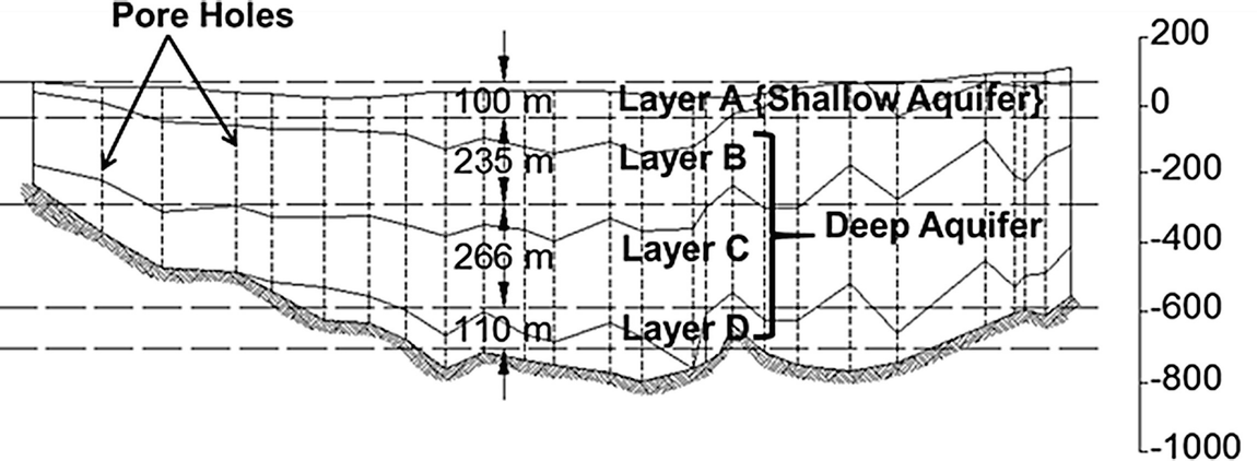
At the Kharga Oasis, [23] classified these water-bearing layers of the average thickness of approximately 700 m into four layers as shown in Fig. 14. In the current study and following [23], the classification and the average thickness of each layer are as follows: (1) layer A with an average thickness of 100 m (top layer), (2) layer B with an average thickness of 235 m, (3) layer C with an average thickness of 266 m and (4) layer D with an average thickness of 110 m (bottom layer). On the basis of this classification, Layer A refers to the shallow aquifer, while the others (layers B, C and D) refer to the deep aquifer.

../images/437178_1_En_84_Chapter/437178_1_En_84_Fig14_HTML.png — Fig. 14
Classification of water-bearing layers compiled from Lamoreaux et al. (1985) [9]

Shata [31] reported that the transmissivity and storage coefficient values for the NSAS under the Kharga Oasis were in the range of 100–2,000 m²/day and 1.5 × 10⁻⁴ to 1.5 × 10⁻², respectively Hesse et al. [41] reported that the hydraulic conductivity of the Kharga part of the NSAS has an average value of 2.16 m/day Ebraheem et al. [18] noted that the average hydraulic conductivity for the regional NSAS is in the range of 0.0864 to 0.864 m/day, with an average storage coefficient of 1.0 × 10⁻⁴. However, these hydraulic properties have not been confirmed for the entire aquifer.

Two types of wells are considered in this study, recent working production wells (RWPWs) and observation wells (OWs). In the current study, the whole area is divided into northern and southern parts. Based on distribution of settlements and RWPW allocations, the studied area was subdivided into eight subdivisions, as shown in Table 1. Table 1 summarizes the name and the available RWPW data for every subdivision. Figure 15 illustrates the locations and distributions of the RWPWs and OWs over the study area. The RWPWs and OWs are distributed over 14% and 45% of the study area, respectively. From Fig. 15, it could be concluded that RWPWs are highly concentrated over two regions: the middle area of the northern part (Area 3–Area 5) and Area 7 in the southern part. For the current study, these two regions were named the M-region and the SN region, respectively. Recent screen depths of the RWPWs range from 76 to 813 m, while the recent depths of the OWs range from 200 to 950 m below the ground surface. Recent groundwater extraction has only been from the deep aquifer (layers B, C and D).

Table 1

Summary of RWPW data throughout subdivisions of the study area

Area no.	Area name	No. of RWPWs	Well depth (m)	Q m³/h
1	Monera	10	101–720	14–117
2	Sherka	11	125–703	14–114
3	Kharga	41	88–706	28–177
4	Jenah	14	89–804	31–329
5	Bulaq	14	163.5–813	46–216
6	Garmashin	12	217–673	20–205
7	Paris	44	76–600	14–229
8	Darb El-Arbeen	41	91.3–485.4	44–56

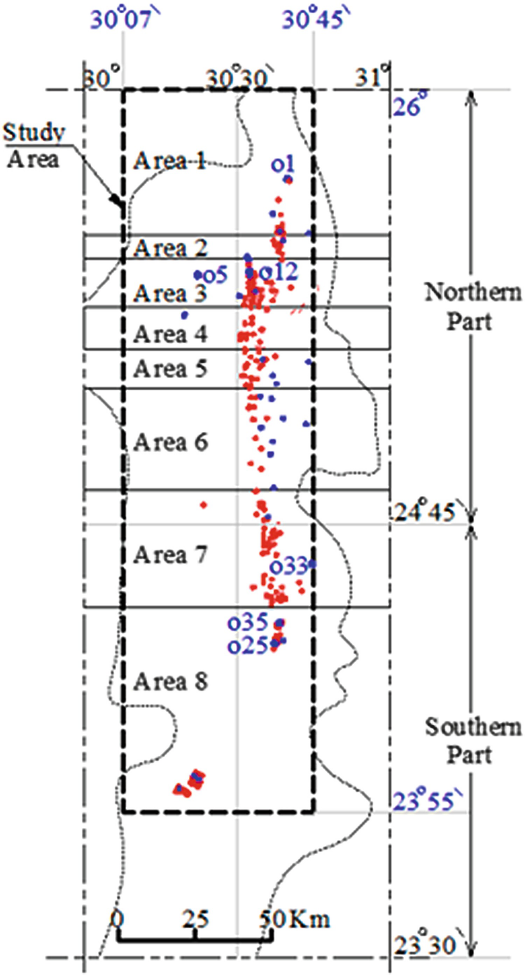
../images/437178_1_En_84_Chapter/437178_1_En_84_Fig15_HTML.png — Fig. 15
Distribution of RWPWs and OWs over the Kharga Oasis; RWPWs shown in *red* and OWs in *blue* [6]. *Dotted line* indicates the schematic boundary of the Kharga Oasis. *Dashed line* indicates the current study area

Q is the discharge from each well

6.1 Hydrogeological Model

Based on the hydrogeological properties of the Kharga Oasis part of the NSAS reported by previous researchers, n hydrogeological models were constructed. For each model, transmissivities (T _xx and T _yy) and storativity values were assumed to be in average ranges of 50–500 m²/day and 3.28 × 10⁻³ to 3.28 × 10⁻², respectively. Although the total discharge extracted from the Kharga Oasis part of the NSAS is known for the period from 1960 to date (Fig. 16), the discharge for each production well within the same period is unknown. For this reason, a scenario of groundwater withdrawal of each RWPW was assumed considering that discharge since 2005 has been almost steady. Groundwater withdrawal for each RWPW was assumed to follow the same groundwater withdrawal trend as the total discharge curve given in Fig. 16. The assumed scenario of groundwater withdrawal started from the year 1960 and increased gradually until the year 2005. Then, it continued steady until 2009. Beyond 2009, three development scenarios of groundwater withdrawal were proposed that involved either expanding the present extraction rate or redistributing the groundwater withdrawal over the recent working production wells (RWPWs) as will be explained later.

../images/437178_1_En_84_Chapter/437178_1_En_84_Fig16_HTML.png — Fig. 16
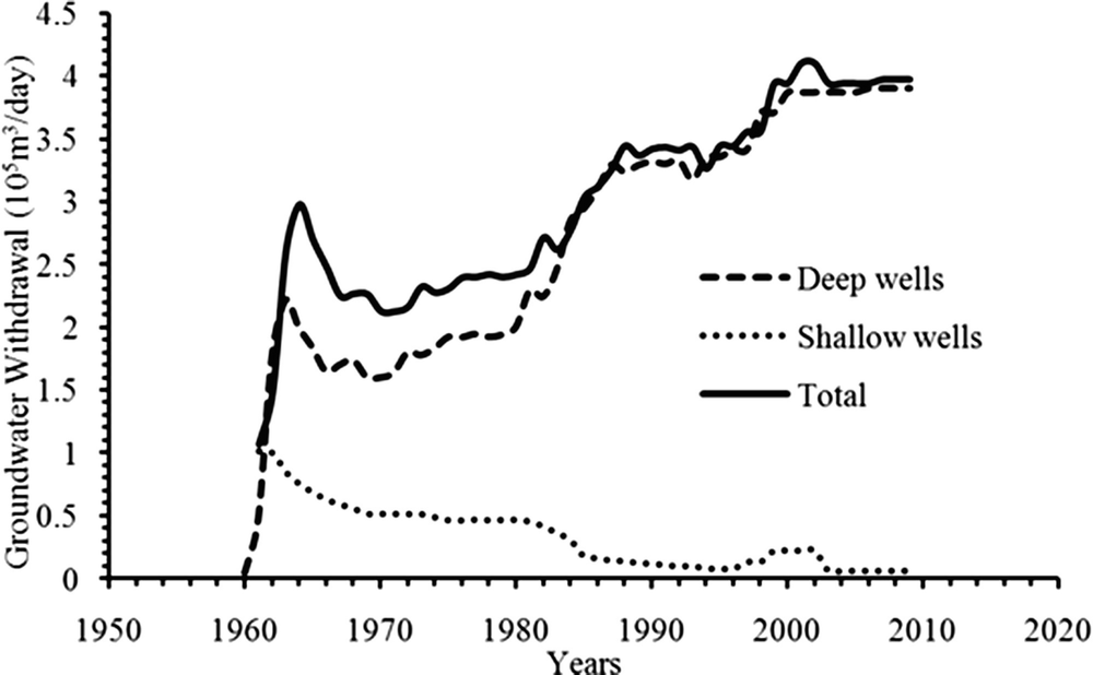
History of groundwater withdrawal from deep and shallow aquifers [4]

6.2 Initial and Boundary Conditions

The NSAS in the Kharga Oasis area is only a small part of the entire NSAS in Egypt. Groundwater flow in the NSAS is governed by the conditions at the boundaries of the regional system. These conditions are not well defined for the Kharga Oasis area. Because of that, the boundary condition was assumed as a fixed boundary head with the flow direction from the southwest to the northeast. With that assumption, the boundary conditions were expressed as hydraulic head values given at the four corners (Z1–Z4) of the calculated area indicated in Fig. 13. Hydraulic heads along each boundary line were assumed to change linearly as shown in Fig. 17. Values of Z1, Z2, Z3 and Z4 were roughly estimated by considering the goodness of fit between the calculated and measured piezometric level trends. In this study, 16 hydrogeological models were assumed with different sets of hydrogeological and boundary conditions as summarized in Table 2.

../images/437178_1_En_84_Chapter/437178_1_En_84_Fig17_HTML.png — Fig. 17
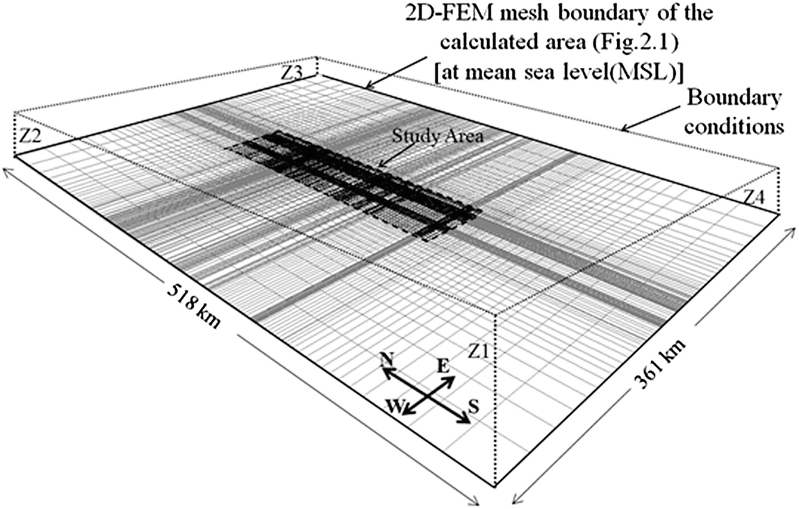
Adopted 2D-FEM mesh geometry for the calculated area, and the study areas. Z1–Z4 are the assumed hydraulic heads at the corners of the calculated area (after six)

Table 2

Proposed hydrogeological models

Model name	Corner hydraulic heads				T _xx (m/day)	T _yy (m/day)	S × 10⁻³
Model name	Z1 (m)	Z2 (m)	Z3 (m)	Z4 (m)	T _xx (m/day)	T _yy (m/day)	S × 10⁻³
M1	87	220	150	105	50	50	32.8
M2	37	170	100	55	50	50	3.28
M3	27	160	90	45	50	500	3.28
M4	37	170	100	55	5	50	3.28
M5	37	170	100	55	500	500	32.8
M6	85	85	85	85	50	500	3.28
M7	37	170	100	100	50	500	3.28
M8	−282	484	123	−111	50	500	3.28
M9	−282	484	123	−90	50	500	3.28
M10	−282	490	123	−111	50	500	3.28
M11	−300	484	123	−111	50	500	3.28
M12	−297	495	108	−126	50	500	3.28
M13	−282	484	123	−111	138	500	3.28
M14	−282	484	123	−111	50	50	3.28
M15	−232	534	123	−61	97	500	3.28
M16	−282	484	123	−111	138	500	32.8

To reduce the direct effects of boundary conditions on the results, the calculated area was extended beyond the study area boundary, as shown in Fig. 13. This area was subdivided into 24,069 rectangular elements and 24,396 nodes with the RWPWs and OWs located on mesh nodes. The elements around the RWPWs and OWs were set as the smallest elements with the sizes gradually increasing towards the boundary of the calculated area, as illustrated in Fig. 17. The minimum and maximum lengths of the element sides were 377 m and 7,000 m, respectively.

6.3 Proposed Future Scenarios for Groundwater Withdrawal

Although the total discharge extracted from the Kharga Oasis part of the NSAS is known from 1960 to 2009 (Fig. 16), the discharge for each production well in the same period is unknown. For this reason, a scenario of groundwater withdrawal of each RWPW was assumed to follow the same groundwater withdrawal trend as the total discharge curve given in Fig. 16, considering that the discharge was almost steady within the period 2005–2009. From 2009 to the present, groundwater withdrawal was assumed to continue being steady. Hereafter, for each RWPW, three scenarios of groundwater withdrawal are assumed, considering that no new production wells will be constructed. The main criterion in the three proposed scenarios is to keep the sum of groundwater withdrawal from the current study area constant. These scenarios are explained as follows:

Scenario 1: The present groundwater withdrawal is increasing and kept constant until the final simulation year of 2100.

Scenario 2: In this scenario, the groundwater withdrawal is redistributed among the RWPWs in the M-region and the southern subdivision Area 8. Area 8 is the highest piezometric level area of the study area [4, 23]. In this scenario, the groundwater withdrawal in the M-region is equal to that in the 1st scenario reduced by 20%. Then, the sum of the groundwater withdrawal reduced from the RWPWs of the M-region is distributed over the RWPWs in Area 8, while keeping the ratio between the RWPW discharges constant.

$\sum {Q}_{\mathrm{M}\hbox{-} \mathrm{region}}=0.80\times \sum {Q}_{\mathrm{M}\hbox{-} \mathrm{region}\left(\mathrm{Scenario}1\right)}$

$\sum {Q}_{\mathrm{Area}7}=\sum {Q}_{\mathrm{Area}8\left(\mathrm{Scenario}1\right)}+0.20\times \sum {Q}_{\mathrm{M}\hbox{-} \mathrm{region}\left(\mathrm{Scenario}1\right)}$

Scenario 3: In this scenario, groundwater withdrawal is redistributed among the RWPWs in the northern part and the southern subdivision Area 8. The groundwater withdrawal of the northern part of this scenario is equal to that in the 1st scenario reduced by 5%. Then, the sum of the groundwater withdrawal reduced from the RWPWs in the northern part is distributed among the RWPWs in Area 8 while keeping the ratio between the RWPW discharges constant:

$\sum {Q}_{\mathrm{Northern}\hbox{-} \mathrm{part}}=0.95\times \sum {Q}_{\mathrm{Northern}\hbox{-} \mathrm{part}\left(\mathrm{Scenario}1\right)}$

$\sum {Q}_{\mathrm{Area}7}=\sum {Q}_{\mathrm{Area}8\left(\mathrm{Scenario}1\right)}+0.05\times \sum {Q}_{\mathrm{M}\hbox{-} \mathrm{region}\left(\mathrm{Scenario}1\right)}$

for which Q is the groundwater withdrawal of each RWPW.

6.4 Sensitivity Analysis

The input parameters population size, crossover probability, mutation probability and number of generations should be properly determined for the proposed MGA model. Moreover, the comparison between the goodness-of-fit values of the MGA and GA models should be analysed under the different values for input parameters. For this purpose, a sensitivity analysis was performed to properly select the appropriate values of these parameters. In this analysis, the measured piezometric level trend at OW o1 was used as a target, and the 16 calculated piezometric level trends calculated by FEM were used as input data for the MGA and GA models. For the GA model, Fig. 18a, b display the relationships among RMSE, number of generations and population size and among RMSE, crossover probability and mutation probability, respectively, and the same for MGA in Fig. 19a, b. From Fig. 18a, it is found that the RMSE value became small with the number of generations = 5,000 and population size ≥100. The relationships among RMSE, crossover probability and mutation probability are more complicated, as displayed in Fig. 18b. It could be concluded that the RMSE became small in the range of 0.70 > crossover probability >0.60 and mutation probability >0.35. On the contrary, Fig. 19a, b show high stability of results in a wide range of parameter values. Considering these results, the selected values of the input parameters for the GA and MGA models are summarized and displayed in Table 3. Consequently, MGA produces a goodness of fit between measured and calculated piezometric levels within a wide range of input parameter values.

../images/437178_1_En_84_Chapter/437178_1_En_84_Fig18_HTML.png — Fig. 18
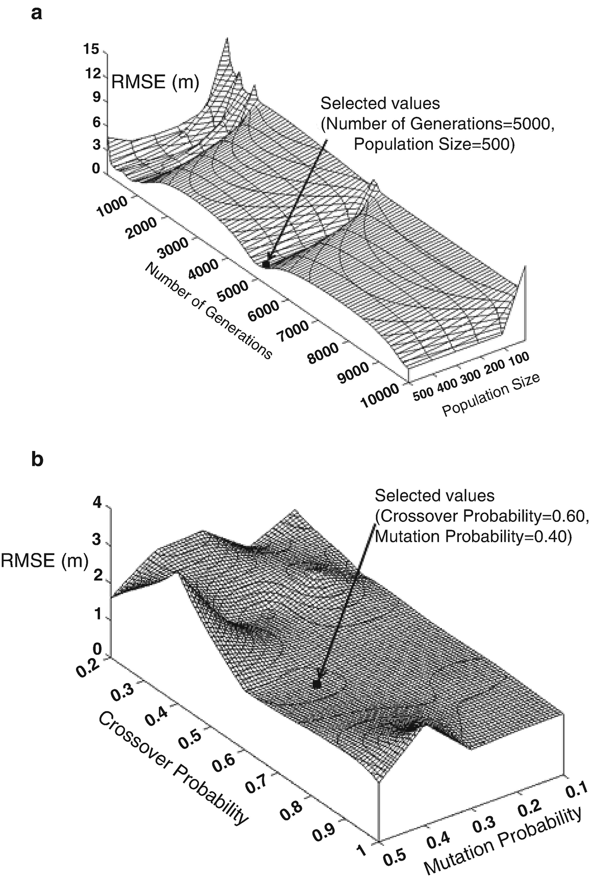
Sensitivity range analysis for the GM: (a) number of generations and population size; (b) crossover and mutation probabilities [6]

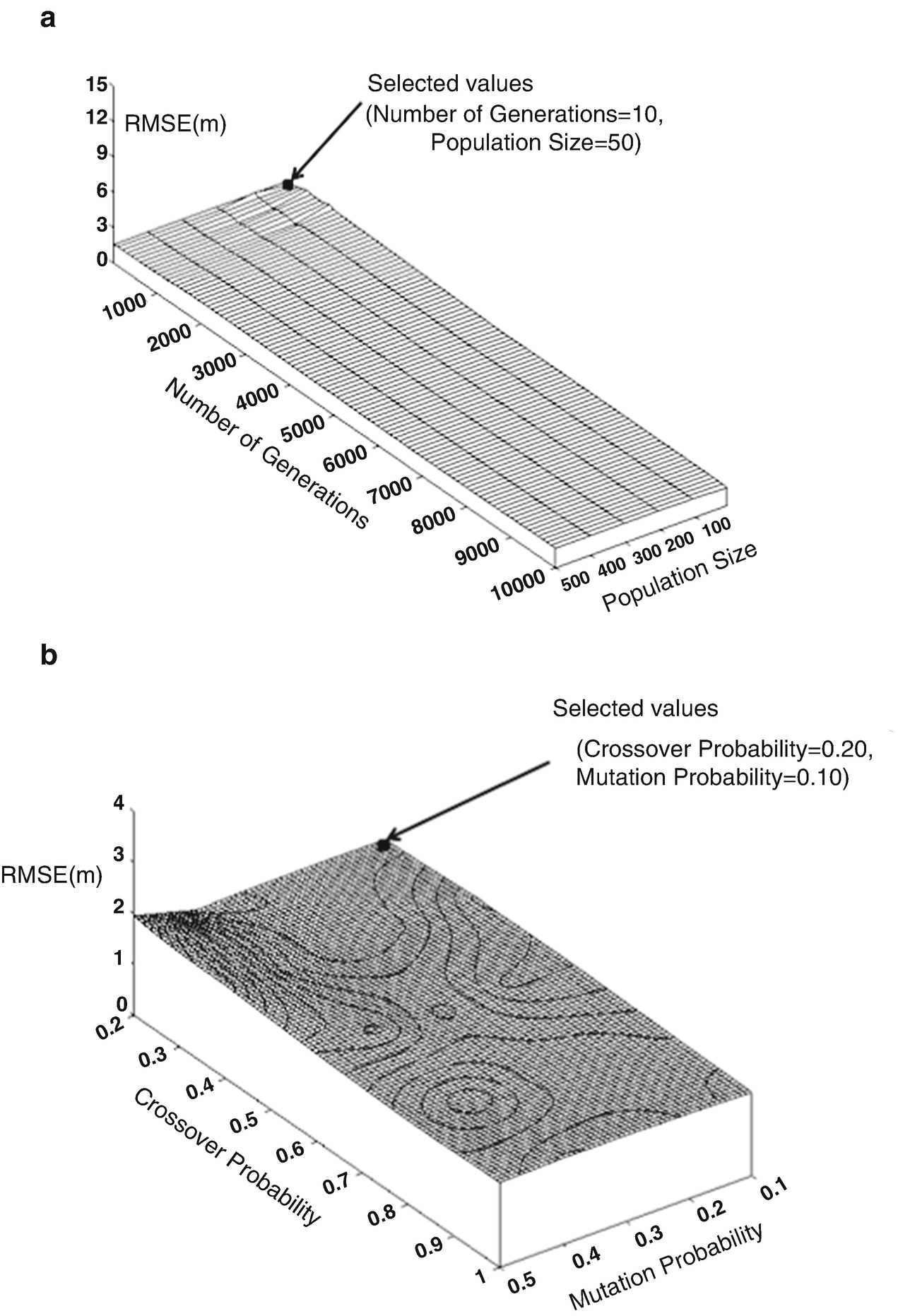
../images/437178_1_En_84_Chapter/437178_1_En_84_Fig19_HTML.png — Fig. 19
Sensitivity range analysis for the MGM: (a) number of generations and population size; (b) crossover and mutation probabilities [9]

Table 3

Setting of GA and MGA models parameters [6]

Parameters	For minimum RMSE		Selected parameters
Parameters	GA	MGA	GA	MGA
Number of generations	5,000	10–10,000	5,000	10
Population size	≥100	10–500	500	50
Crossover probability	0.60–0.70	0.2–1.0	0.60	0.20
Mutation probability	≥0.35	0.1–0.4	0.40	0.10

6.5 Future Assessment of Temporal Piezometric Level Change

The good agreement between the measured and calculated piezometric level trends in the short period simulation (1979–2005) was considered to be a verification of the MGM presented in this study. Thus, the MGM can be used to predict piezometric level trends and drawdown of the groundwater table over long periods, as well as to evaluate the hydrological feasibility of the proposed groundwater withdrawal plans (scenarios 1, 2 and 3). With regards to the proposed scenarios for groundwater withdrawal described previously, the simulated declines in hydraulic head at the target OWs were calculated for the period 1960 to 2100.

For the proposed scenarios of groundwater withdrawal (scenario 1, scenario 2 and scenario 3), Figs. 20, 21 and 22 show the simulated piezometric levels of the target OWs, respectively. For scenario 1, Fig. 20 shows the piezometric level trends simulated by the MGM and that previously simulated by the GM [4] for the target OWs. From this figure, both models simulating the piezometric level trends are highly correlated, which confirms the validity of the newly developed MGM for future assessment of hydraulic heads. However, the MGM input parameters values are smaller than those of GM. The results indicate that the MGM produced satisfactory validation results compared to the ordinary GM considering the use of a small number of inputs and the low values of the input parameters. Moreover, the time required for calculations, represented by the number of generations parameter, is reduced from 5,000 for the GM to 10 for the MGM, which is a considerably large reduction of 99.98%.

../images/437178_1_En_84_Chapter/437178_1_En_84_Fig20_HTML.png — Fig. 20
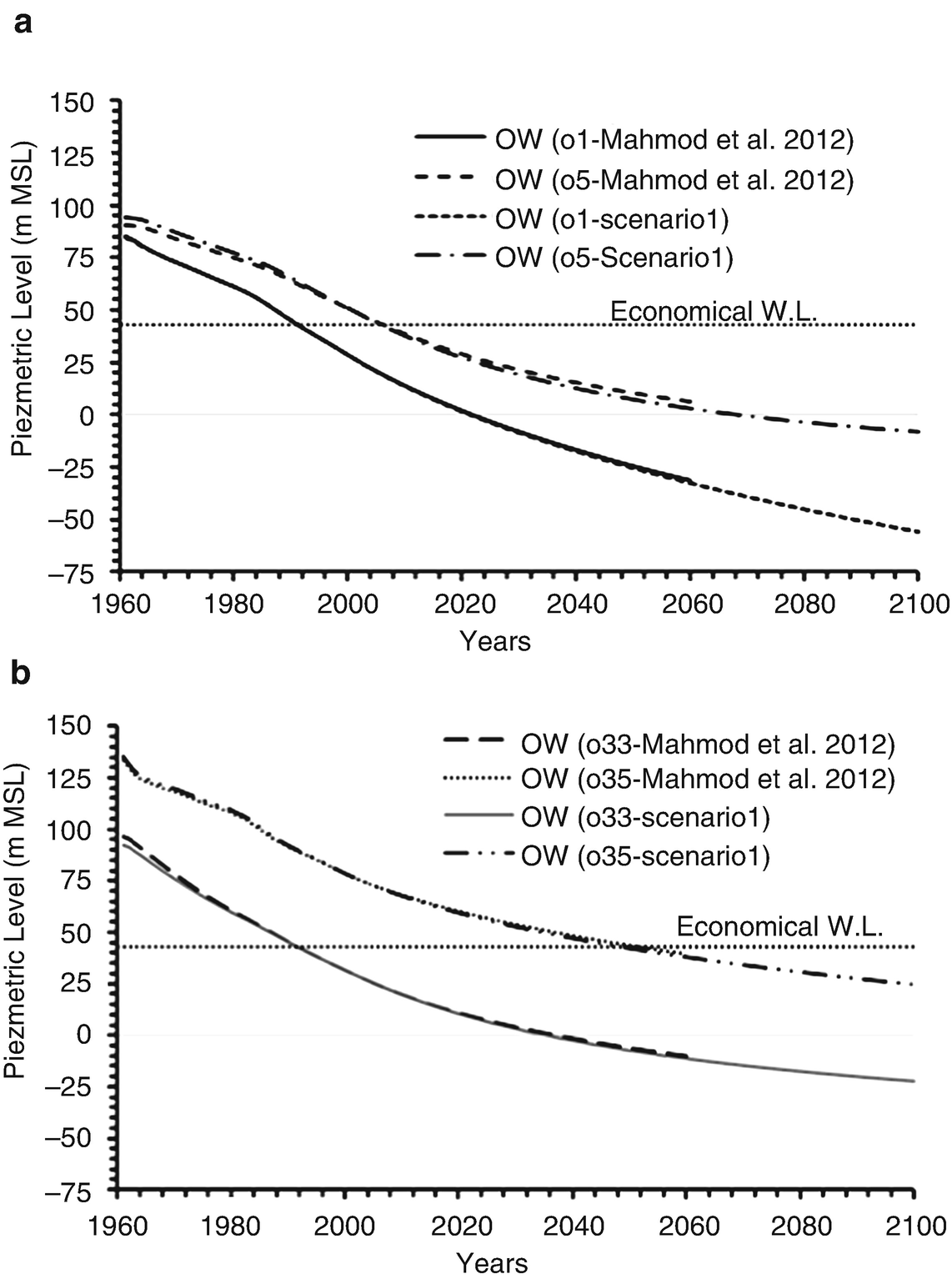
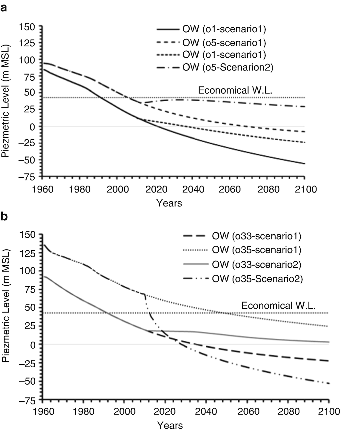
Comparison of simulated piezometric levels for MGM and GM [39] until the year 2100: (a) OWs o1 and o5; (b) OWs o33 and o35 [6]

../images/437178_1_En_84_Chapter/437178_1_En_84_Fig21_HTML.png — Fig. 21
Comparison of MGM-simulated piezometric levels for scenario 2 and scenario 1 until the year 2100: (a) OWs o1 and o5; (b) OWs o33 and o35 [6]

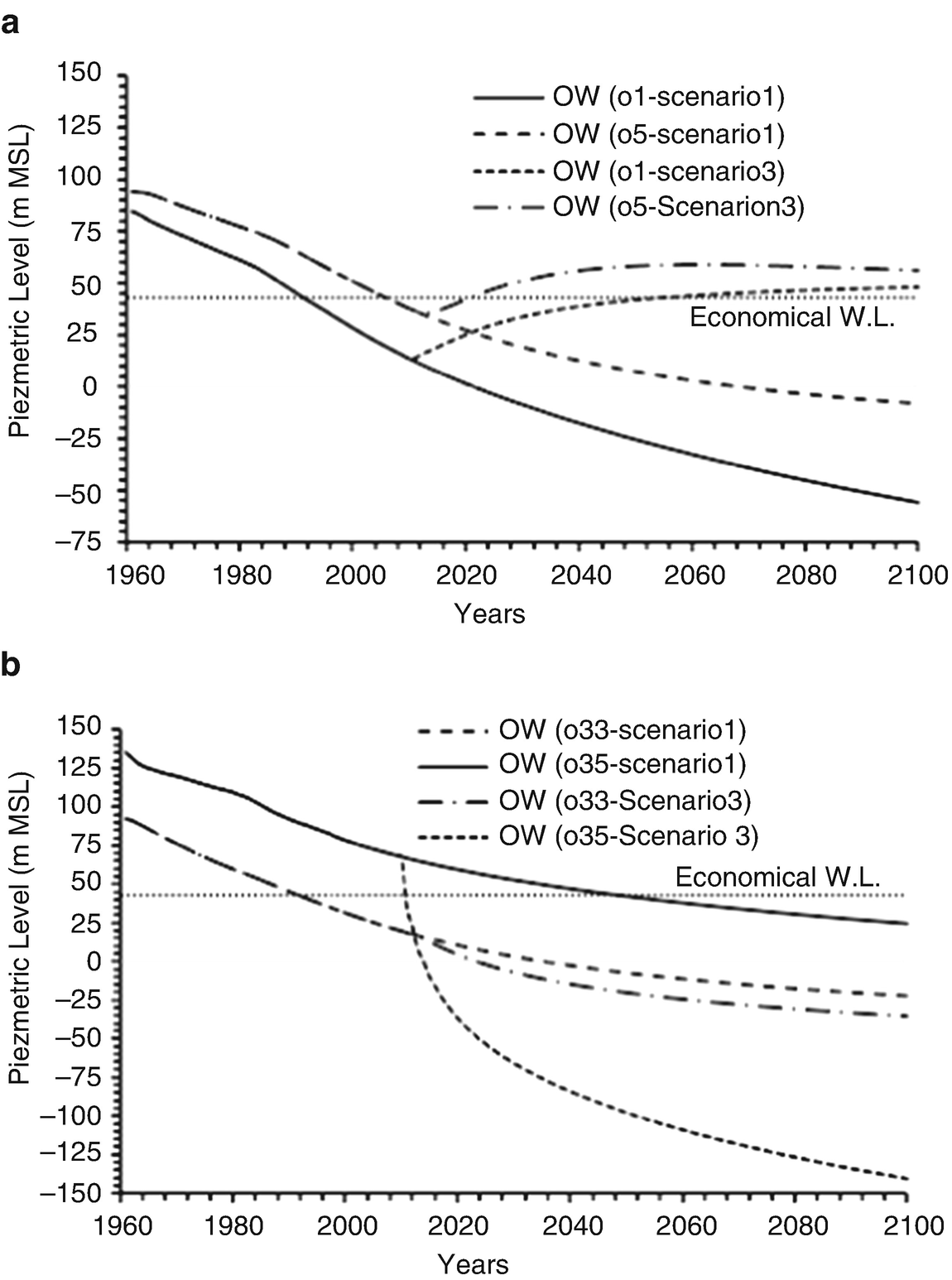
../images/437178_1_En_84_Chapter/437178_1_En_84_Fig22_HTML.png — Fig. 22
Comparison of MGM-simulated piezometric levels for scenario 3 and scenario 1 until the year 2100: (a) OWs o1 and o5; (b) OWs o33 and o35 [6]

For scenario 2, Fig. 21 shows that the hydraulic heads of OWs o1, o5 and o33 are recovered by 32.0, 37.5 and 25.0 m, respectively, compared to those in scenario 1. On the contrary, the hydraulic head of OW o35 is severely decreased by 77.8 m. Comparing scenario 3 with scenario 1, Fig. 22 shows that the hydraulic heads of OWs o1 and o5 are recovered by 104.0 and 64.5 m, respectively, to reach their economical piezometric levels by the years 2039 and 2018. On the other hand, the hydraulic heads of OWs o33 and o35 are decreased by 13 and 165 m, respectively. For both scenarios 2 and 3, the high decrease in hydraulic head of OW o35 as a representative of Area 8 is due to the high groundwater withdrawal that added to the RWPWs in this area. Therefore, it is recommended to drill new production wells in the southern part of the study area to reduce groundwater withdrawal over the RWPWs. For the three scenarios, Table 4 shows the differences in hydraulic heads between the economical piezometric head levels and the target OWs’ piezometric levels beyond 2100. A positive sign indicates that the piezometric level of the OW is above the economical one and vice versa.

Table 4

Hydraulic head differences in the economical piezometric levels for the target OWs

OW	Difference from the economical piezometric level (43 m) by 2100
OW	Scenario 1	Scenario 2	Scenario 3
o1	−98.88	−66.89	4.98
o5	−51.16	−13.58	13.27
o33	−65.22	−39.76	−78.26
o35	−18.33	−96.08	−183.62

The MGM shows a better fitting performance than the ordinary GM, for which the best input models’ trends are recognized by means of the best models combination (BMC_k). On the other hand, the MGM produced a wide range of input parameter values, which guarantees goodness of fit with any hypothetical value of these parameters. Moreover, a high reduction in required calculation time was observed for reaching the best fit to the observations.

6.6 Evaluation of the Proposed Groundwater Withdrawal Scenarios

As a trial to evaluate the proposed scenarios of groundwater withdrawal, a contour map of hydraulic head distributions was constructed to understand the future hydrogeological conditions of groundwater flow in the study area. Figure 23a–c show the flow direction and hydraulic head distributions for the three proposed scenarios, scenario 1, scenario 2 and scenario 3 for year 2100, respectively. From these figures, it could be concluded that the hydraulic heads of the northern part could be recovered as well as the hydraulic head of point P1 for the three scenarios; scenario 1, scenario 2 and scenario 3 have the values of −60, 0, and 50 m, respectively. On the other hand, for the southern part, the hydraulic head of point P2 for the same three scenarios is 80, 20, and −100 m respectively. The drawdown which occurred at the southern part (Area 8) was due to the small number of RWPWs that were used in the redistribution process of groundwater withdrawal. By comparing the hydraulic heads at points P1 and P2, which are representative of the northeastern and southwestern parts of the study area, respectively, it could be concluded that the differences in hydraulic heads between these two points were 140, 20, and −150 m for the three scenarios: scenario 1, scenario 2 and scenario 3, respectively. The negative sign here is a result of a decrease in the piezometric level of point P2 comparing with that of point P1 because of small number of RWPWs in the southern part (Area 8). The percentage of the whole currently affected study area for the three scenarios scenario 1, scenario 2 and scenario 3 at year 2100 are 80%, 70% and 50%, respectively. In general, a recovery of the hydraulic head distribution could be achieved by redistribution of the groundwater withdrawal of the RWPWs. Consequently, the northern part of the study area could be highly recovered for the three proposed scenarios, as well as a high recovery percentage of the whole area was achieved by applying scenario 3 (50% recovered) with a recommendation of increase in the number of RWPWs at the southern part of the study area (Area 8).

../images/437178_1_En_84_Chapter/437178_1_En_84_Fig23_HTML.png — Fig. 23
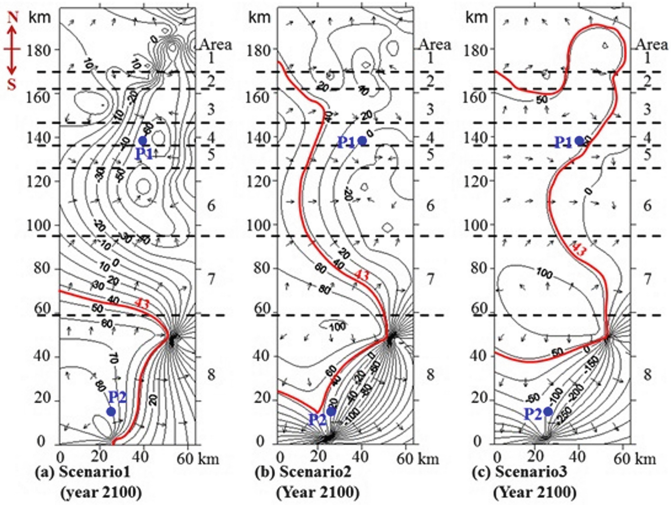
Comparison between the simulated piezometric level contours along with groundwater flow vectors in the study area for the proposed scenarios [9]

7 Conclusions

In this study, groundwater flow analysis was performed using the developed modified grey model (MGM) which combines the finite element method (FEM) and the new developed modified genetic algorithm (MGA). The analysis of observed data shows enormous pore pressure decrease by 50 m in the northeastern part of the study area within the period 1979–2005. The MGM produced stable results for piezometric level simulations while using a wide range of input parameters values compared to the ordinary grey model (GM). Moreover, the time required for calculations to achieve proper convergence with the measured piezometric level trends was reduced by 99.8% compared to the GM. MGM used a smaller number of input models’ trends than the GM for achieving goodness of fit, with a percentage of reduction in the range of 68.75–81.25%. The RMSE was in the ranges of 0.63–2.936 m and 0.439–2.665 for the MGM and the GM, respectively. The results from the various scenarios of groundwater withdrawal demonstrate that if the present extraction rate is expanded (scenario 1), the groundwater piezometric level continuously declines and drops below the economical piezometric level until the year 2100 at the end of the simulation period. To avoid groundwater depletion in the Kharga Oasis, the extraction rate in the M-region is lowered by 20% and added to Area 8 (scenario 2). The planned extraction rate is not feasible for the future and will have a negative impact on the piezometric level of Area 8. However, a recovery in the piezometric levels for all other subdivisions was observed. For the 3rd scenario of groundwater withdrawal, the recovery head for the northern area increased more than in scenario 2, as well as reached above the economical piezometric level. However, a large drawdown of the piezometric level of the southern part was observed.

8 Recommendations

To protect the groundwater table from being severely drawn down, it is recommended that new production wells be constructed in the southern part of the current study area far enough from the RWPWs. For reliable piezometric measurements, a network of monitoring wells should be drilled that cover the whole area. Regular water-level measurements (at least monthly) would provide the basic data needed for time series compilations in the future, which could give feedback on the constructed model. For the future, it is suggested that the MGM be used for simulating the total piezometric level surface of the whole area and hence confirm the MGM performance. The proposed model (MGM) is significant for the decision-makers to have knowledge about groundwater resources in their regions. For that, MGM could be useful to study the effect of increased pressure on the finite water resource on the sustainability of agricultural production and livelihoods as well as the social cohesion within new settler communities. Moreover, a new developed monitoring system could be proposed to reduce the monitoring cost based on giving up the idea of constructing new observation wells.

References

1.
El Tahlawi MR, Farrag AA, Ahmed SS (2008) Groundwater of Egypt: “an environmental overview”. Environ Geol 55:639–652Crossref
2.
Elbeih SF (2015) An overview of integrated remote sensing and GIS for groundwater mapping in Egypt. Ain Shams Eng J 6:1–15Crossref
3.
UNESCO (2013) Joint programme for climate change risk management in Egypt – proposed climate change adaptation strategy for the Ministry of Water Resources & Irrigation Egypt. Ministry of Water Resources and Irrigation
4.
Mahmod WE, Watanabe K, Zahr-Eldeen AA (2013) Analysis of groundwater flow in arid areas with limited hydrogeological data using the Grey model: a case study of the Nubian Sandstone, Kharga Oasis, Egypt. Hydrgeol J 21:1021–1034Crossref
5.
El Arabi N (2012) Environmental management of groundwater in Egypt via artificial recharge extending the practice to soil aquifer treatment (SAT). Int J Environ Sustain 1(3):66–82Crossref
6.
Mahmod WE, Watanabe K (2014) Modified Grey model and its application to groundwater flow analysis with limited hydrogeological data: a case study of the Nubian Sandstone, Kharga Oasis, Egypt. Environ Monit Assess J 186:1063–1081Crossref
7.
Idris H, Nour S (1990) Present groundwater status in Egypt and the environmental impacts. Environ Geol Water Sci 16(3):171–177Crossref
8.
Alnaggar D (2003) Water resources management and policies for Egypt. Workshop on policies and strategies options for water management in Islamic countries, Tehran; December
9.
Mahmod WE (2016) Modeling of complex groundwater flow systems using MGM. LAP Lambert Academic Publishing, 128 p
10.
RIGW/IWACO (1988) Hydrogeological mapping of Egypt, scale 1:2,000,000. 1st edn. TN 70.120-88-03, http://earthwise.bgs.ac.uk/index.php/Hydrogeology_of_Egypt
11.
Allam AR, Ele-Jan S, Dawoud MA (2002) Desalination of brackish groundwater in Egypt. Desalination 152:19–26Crossref
12.
Dawoud MA (2004) Design of national groundwater quality monitoring network in Egypt. Environ Monit Assess 96:99–1180Crossref
13.
Hefny K, Shata A (2004) Underground water in Egypt. Ministry of water supplies and irrigation, Cairo, Egypt, p 295 (in Arabic)
14.
Armanuos AM, Ibrahim MG, Mahmod WE, Negm, A, Yoshimura C, Jiro Takemura J, Zidan BA (2017) Evaluation the potential impact of Grand Ethiopian Renaissance Dam and pumping scenarios on groundwater level in the Nile Delta aquifer, Water Science & Technology: Water Supply. doi:10.2166/ws.2017.037
15.
Ambroggi RP (1966) Water under the Sahara. Sci Am 214:21–29Crossref
16.
Hefny K, Shata A (1995) Strategies for planning and management of groundwater in the Nile Valley and Delta in Egypt. Strategic research program-working paper series no. 31-1. Environmental and Natural Resources Policy and Training Project (EPAT)
17.
Ebraheem AM, Garamoon HK, Wycisk P, Seif El Nasr AM (2003) Numerical modeling of groundwater resource management options in the East Oweinat area, SW Egypt. Environ Geol 44:433–447Crossref
18.
Ebraheem AM, Riad S, Wycisk P, Seif El Nasr AM (2002) Simulation of impact of present and future groundwater extraction from the non-replenished Nubian Sandstone Aquifer in SW Egypt. Environ Geol 43:188–196Crossref
19.
Heinl M, Thorweihe U (1993) Groundwater resources and management in SW Egypt. In: Meissner B, Wycisk P (eds) Geopotential and ecology. Catena Suppl 26:99–121
20.
Ball J (1927) Problems of the Libyan desert. Geogr J 70:21–38, 105–128, 209–224Crossref
21.
Sanford KS (1935) Source of water in the northern-western Sudan. Geogr J 85:412–431Crossref
22.
Sonntag C (1986) A time-dependent groundwater model for the Eastern Sahara. Berl Geowiss Abh A72:124–134
23.
Lamoreaux PE, Memon BA, Idris H (1985) Groundwater development, Kharga Oasis, western desert of Egypt: along-term environment concern. Environ Geol Water Sci 7:129–149Crossref
24.
Masoud MH, Schneider M, El Osta MM (2013) Recharge flux to the Nubian Sandstone aquifer and its impact on the present development in southwest Egypt. Journal of African Earth Science 85:115–124Crossref
25.
Thorweihe U, Heinl M (2002) Groundwater resources of the Nubian aquifer system, NE-Africa. Synthesis, Observatoire du Sahara et du Sahel, Paris
26.
Knetsch G, Yallouze M (1955) Remarks on the origin of the Egyptian Oasis depressions. Bull Soc Géogr Égypte 28:21–33
27.
Said R (1962) The geology of Egypt. Elsevier, Amsterdam
28.
Said R (1990) Geomorphology. In: Said R (ed) The geology of Egypt. Tailor & Francis, Rotterdam
29.
Thorweihe U, Schandelmeier H (1993) Geoscientific research in Northeast Africa. Proceedings of international conference on geoscience. A.A. Balkema, Rotterdam, 776 p
30.
Thorweihe U (1990) The Nubian aquifer system. In: Said R (ed) The geology of Egypt, Balkema, Lisse, The Netherlands, pp 601–614
31.
Shata AA (1982) Hydrogeology of the great Nubian Sandstone basin, Egypt. Q J Eng Geol 15:127–133Crossref
32.
Mohammed M, Watanabe K, Takeuchi S (2010) Grey model for prediction of pore pressure change. Environ Earth Sci 60:1523–1534Crossref
33.
Anderson MP, Woessener WW (1992) Applied groundwater modeling-simulation of flow and advective transport. Academic Press Inc, San Diego
34.
Pinder GF, Gray WG (1977) Finite element simulation in surface and subsurface hydrology. Academic Press Inc, New York
35.
Sivaraj R (2011) A review of selection methods in genetic algorithm. Int J Eng Technol 3:3792–3797
36.
Goldberg DE, Deb K (1991) A comparative analysis of selection schemes used in genetic algorithms. In: Rawlins GJE (ed) Foundations of genetic algorithms. Morgan Kaufmann Publishers Inc, San Francisco, CA
37.
Mitchell M (1999) An introduction to genetic algorithms, 5th printing. Massachusetts Institute of Technology, London
38.
Coley DA (1999) An introduction to genetic algorithms for scientists and engineers. World Scientific Publishing Co Pte Ltd, SingaporeCrossref
39.
Mahmod WE, Watanabe K (2012) A preliminary modification and validation of the Grey Model for groundwater flow analysis of arid regions, VII international conference on environmental hydrology, Egypt
40.
Salman AB, Howari FM, El-Sankary MM, Wali AM, Saleh MM (2010) Environmental impact and natural hazards on Kharga Oasis monumental sites, Western Desert of Egypt. J African Earth Sci 58:341–353Crossref
41.
Hesse K, Hissne A, Kheir O, Schnäcker E, Schneider M, Thorweihe U (1987) Hydrogeological investigations in the Nubian sandstone aquifer system, Eastern Sahara. Berl Geowiss Abh A75:397–4641