The goal of data analytics in general is to uncover actionable insights that result in positive business outcomes. In the case of predictive analytics, the aim is to do this by determining the most likely future outcome of a target, based on previous trends and patterns.
The benefits of predictive analytics are not restricted to big technology companies. Any business can find ways to benefit from machine learning, given the right data.
Companies all around the world are collecting massive amounts of data and using predictive analytics to cut costs and increase profits. Some of the most prevalent examples of this are from the technology giants Google, Facebook, and Amazon, who utilize big data on a huge scale. For example, Google and Facebook serve you personalized ads based on predictive algorithms that guess what you are most likely to click on. Similarly, Amazon recommends personalized products that you are most likely to buy, given your previous purchases.
Modern predictive analytics is done with machine learning, where computer models are trained to learn patterns from data. As we saw briefly in the previous lesson, software such as scikit-learn can be used with Jupyter Notebooks to efficiently build and test machine learning models. As we will continue to see, Jupyter Notebooks are an ideal environment for doing this type of work, as we can perform ad hoc testing and analysis, and easily save the results for reference later.
In this lesson, we will again take a hands-on approach by running through various examples and activities in a Jupyter Notebook. Where we saw a couple of examples of machine learning in the previous lesson, here we'll take a much slower and more thoughtful approach. Using an employee retention problem as our overarching example for the lesson, we will discuss how to approach predictive analytics, what things to consider when preparing the data for modeling, and how to implement and compare a variety of models using Jupyter Notebooks.
- Plan a machine learning classification strategy
- Preprocess data to prepare it for machine learning
- Train classification models
- Use validation curves to tune model parameters
- Use dimensionality reduction to enhance model performance
Here, we will cover the preparation required to train a predictive model. Although not as technically glamorous as training the models themselves, this step should not be taken lightly. It's very important to ensure you have a good plan before proceeding with the details of building and training a reliable model. Furthermore, once you've decided on the right plan, there are technical steps in preparing the data for modeling that should not be overlooked.
Note
We must be careful not to go so deep into the weeds of technical tasks that we lose sight of the goal.
Technical tasks include things that require programming skills, for example, constructing visualizations, querying databases, and validating predictive models. It's easy to spend hours trying to implement a specific feature or get the plots looking just right. Doing this sort of thing is certainly beneficial to our programming skills, but we should not forget to ask ourselves if it's really worth our time with respect to the current project.
Also, keep in mind that Jupyter Notebooks are particularly well-suited for this step, as we can use them to document our plan, for example, by writing rough notes about the data or a list of models we are interested in training. Before starting to train models, it's good practice to even take this a step further and write out a well-structured plan to follow. Not only will this help you stay on track as you build and test the models, but it will allow others to understand what you're doing when they see your work.
After discussing the preparation, we will also cover another step in preparing to train the predictive model, which is cleaning the dataset. This is another thing that Jupyter Notebooks are well-suited for, as they offer an ideal testing ground for performing dataset transformations and keeping track of the exact changes. The data transformations required for cleaning raw data can quickly become intricate and convoluted; therefore, it's important to keep track of your work. As discussed in the first lesson, tools other than Jupyter Notebooks just don't offer very good options for doing this efficiently.
When formulating a plan for doing predictive modeling, one should start by considering stakeholder needs. A perfect model will be useless if it doesn't solve a relevant problem. Planning a strategy around business needs ensures that a successful model will lead to actionable insights.
Although it may be possible in principle to solve many business problems, the ability to deliver the solution will always depend on the availability of the necessary data. Therefore, it's important to consider the business needs in the context of the available data sources. When data is plentiful, this will have little effect, but as the amount of available data becomes smaller, so too does the scope of problems that can be solved.
These ideas can be formed into a standard process for determining a predictive analytics plan, which goes as follows:
- Look at the available data to understand the range of realistically solvable business problems. At this stage, it might be too early to think about the exact problems that can be solved. Make sure you understand the data fields available and the timeframes they apply to.
- Determine the business needs by speaking with key stakeholders. Seek out a problem where the solution will lead to actionable business decisions.
- Assess the data for suitability by considering the availability of a sufficiently diverse and large feature space. Also, take into account the condition of the data: are there large chunks of missing values for certain variables or time ranges?
Steps 2 and 3 should be repeated until a realistic plan has taken shape. At this point, you will already have a good idea of what the model input will be and what you might expect as output.
Once we've identified a problem that can be solved with machine learning, along with the appropriate data sources, we should answer the following questions to lay a framework for the project. Doing this will help us determine which types of machine learning models we can use to solve the problem:
- Is the training data labeled with the target variable we want to predict?
If the answer is yes, then we will be doing supervised machine learning. Supervised learning has many real-world use cases, whereas it's much rarer to find business cases for doing predictive analytics on unlabeled data.
If the answer is no, then you are using unlabeled data and hence doing unsupervised machine learning. An example of an unsupervised learning method is cluster analysis, where labels are assigned to the nearest cluster for each sample.
- If the data is labeled, then are we solving a regression or classification problem?
In a regression problem, the target variable is continuous, for example, predicting the amount of rain tomorrow in centimeters. In a classification problem, the target variable is discrete and we are predicting class labels. The simplest type of classification problem is binary, where each sample is grouped into one of two classes. For example, will it rain tomorrow or not?
- What does the data look like? How many distinct sources?
Consider the size of the data in terms of width and height, where width refers to the number of columns (features) and height refers to the number of rows. Certain algorithms are more effective at handling large numbers of features than others. Generally, the bigger the dataset, the better in terms of accuracy. However, training can be very slow and memory intensive for large datasets. This can always be reduced by performing aggregations on the data or using dimensionality reduction techniques.
If there are different data sources, can they be merged into a single table? If not, then we may want to train models for each and take an ensemble average for the final prediction model. An example where we may want to do this is with various sets of times series data on different scales. Consider we have the following data sources: a table with the AAPL stock closing prices on a daily time scale and iPhone sales data on a monthly time scale.
We could merge the data by adding the monthly sales data to each sample in the daily time scale table, or grouping the daily data by month, but it might be better to build two models, one for each dataset, and use a combination of the results from each in the final prediction model.
Data preprocessing has a huge impact on machine learning. Like the saying "you are what you eat," the model's performance is a direct reflection of the data it's trained on. Many models depend on the data being transformed so that the continuous feature values have comparable limits. Similarly, categorical features should be encoded into numerical values. Although important, these steps are relatively simple and do not take very long.
Another thing to consider is the size of the datasets being used by many data scientists. As the dataset size increases, the prevalence of messy data increases as well, along with the difficulty in cleaning it.
Simply dropping the missing data is usually not the best option, because it's hard to justify throwing away samples where most of the fields have values. In doing so, we could lose valuable information that may hurt final model performance.
The steps involved in data preprocessing can be grouped as follows:
- Merging data sets on common fields to bring all data into a single table
- Feature engineering to improve the quality of data, for example, the use of dimensionality reduction techniques to build new features
- Cleaning the data by dealing with duplicate rows, incorrect or missing values, and other issues that arise
- Building the training data sets by standardizing or normalizing the required data and splitting it into training and testing sets
Let's explore some of the tools and methods for doing the preprocessing.
- Start the
NotebookAppfrom the project directory by executingjupyter notebook. Navigate to theLesson-2directory and open up thelesson-2-workbook.ipynbfile. Find the cell near the top where the packages are loaded, and run it.We are going to start by showing off some basic tools from Pandas and scikit-learn. Then, we'll take a deeper dive into methods for rebuilding missing data.
- Scroll down to
Subtopic B: Preparing data for machine learningand run the cell containingpd.merge?to display the docstring for themergefunction in the notebook: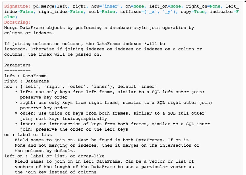
As we can see, the function accepts a left and right DataFrame to merge. You can specify one or more columns to group on as well as how they are grouped, that is, to use the left, right, outer, or inner sets of values. Let's see an example of this in use.
- Exit the help popup and run the cell containing the following sample DataFrames:
df_1 = pd.DataFrame({'product': ['red shirt', 'red shirt', 'red shirt', 'white dress'],\n",
                     'price': [49.33, 49.33, 32.49, 199.99]})\n",
df_2 = pd.DataFrame({'product': ['red shirt', 'blue pants', 'white tuxedo', 'white dress'],\n",
                     'in_stock': [True, True, False, False]})
Here, we will build two simple DataFrames from scratch. As can be seen, they contain a
productcolumn with some shared entries.Now, we are going to perform an inner merge on the
productshared column and print the result. - Run the next cell to perform the inner merge:
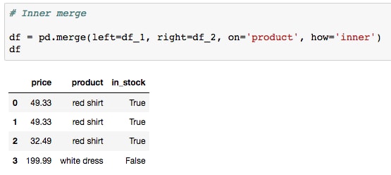
Note how only the shared items, red shirt and white dress, are included. To include all entries from both tables, we can do an outer merge instead. Let's do this now.
- Run the next cell to perform an outer merge:
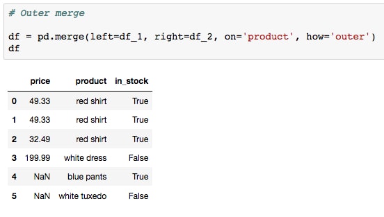
This returns all of the data from each table where missing values have been labeled with
NaN. - Run the next cell to perform an outer merge:
This returns all of the data from each table where missing values have been labeled with
NaN.
Since this is our first time encountering an NaN value in this book, now is a good time to discuss how these work in Python.
First of all, you can define an NaN variable by doing, for example, a = float('nan'). However, if you want to test for equality, you cannot simply use standard comparison methods. It's best to do this instead with a high-level function from a library such as NumPy. This is illustrated with the following code:
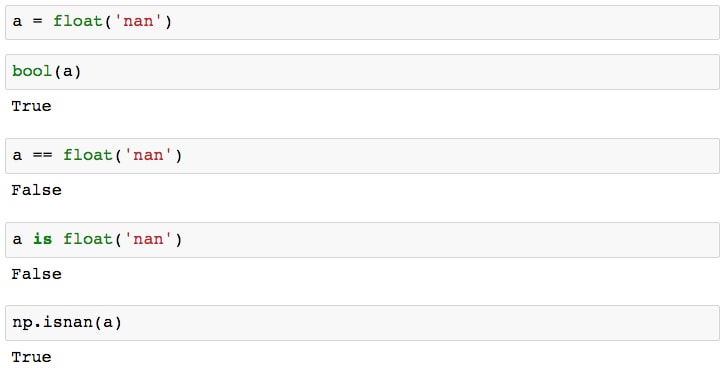
Some of these results may seem counterintuitive. There is logic behind this behavior, however, and for a deeper understanding of the fundamental reasons for standard comparisons returning False, check out this excellent StackOverflow thread: https://stackoverflow.com/questions/1565164/what-is-the-rationale-for-all-comparisons-returning-false-for-ieee754-nan-values.
- You may have noticed that our most recently merged table has duplicated data in the first few rows. Let's see how to handle this.
Run the cell containing
df.drop_duplicates()to return a version of the DataFrame with no duplicate rows: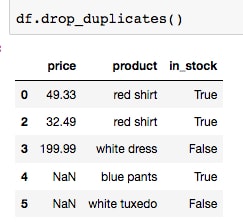
This is the easiest and "standard" way to drop duplicate rows. To apply these changes to
df, we can either setinplace=Trueor do something likedf = df.drop_duplicated(). Let's see another method, which uses masking to select or drop duplicate rows. - Run the cell containing
df.duplicated()to print the True/False series, marking duplicate rows: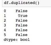
We can take the sum of this result to determine how many rows have duplicates, or it can be used as a mask to select the duplicated rows.
- Do this by running the next two cells:

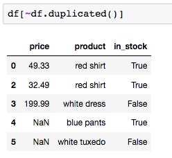
- We can compute the opposite of the mask with a simple tilde (
~) to extract the deduplicatedDataFrame. Run the following code and convince yourself the output is the same as that fromdf.drop_duplicates():df[~df.duplicated()]
- This can also be used to drop duplicates from a subset of the full DataFrame. For example, run the cell containing the following code:
df[~df['product'].duplicated()]
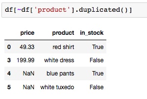
Here, we are doing the following things:
- Creating a mask (a True/False series) for the product row, where duplicates are marked with
True - Using the tilde (
~) to take the opposite of that mask, so that duplicates are instead marked withFalseand everything else isTrue - Using that mask to filter out the
Falserows ofdf, which correspond to the duplicated products
As expected, we now see that only the first red shirt row remains, as the duplicate product rows have been removed.
In order to proceed with the steps, let's replace
dfwith a deduplicated version of itself. This can be done by runningdrop_duplicatesand passing the parameterinplace=True. - Creating a mask (a True/False series) for the product row, where duplicates are marked with
- Deduplicate the DataFrame and save the result by running the cell containing the following code:
df.drop_duplicates(inplace=True)
Continuing on to other preprocessing methods, let's ignore the duplicated rows and first deal with the missing data. This is necessary because models cannot be trained on incomplete samples. Using the missing price data for blue pants and white tuxedo as an example, let's show some different options for handling
NaNvalues. - One option is to drop the rows, which might be a good idea if your
NaNsamples are missing the majority of their values. Do this by running the cell containingdf.dropna():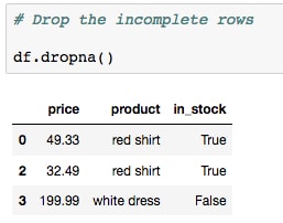
- If most of the values are missing for a feature, it may be best to drop that column entirely. Do this by running the cell containing the same method as before, but this time with the axes parameter passed to indicate columns instead of rows:
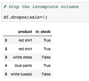
Simply dropping the
NaNvalues is usually not the best option, because losing data is never good, especially if only a small fraction of the sample values is missing. Pandas offers a method for filling inNaNentries in a variety of different ways, some of which we'll illustrate now. - Run the cell containing
df.fillna?to print the docstring for the PandasNaN-fillmethod:
Note the options for the
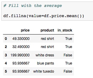
valueparameter; this could be, for example, a single value or a dictionary/series type map based on index. Alternatively, we can leave the value asNoneand pass afillmethod instead. We'll see examples of each in this lesson. - Fill in the missing data with the average product price by running the cell containing the following code:
df.fillna(value=df.price.mean())
- Now, fill in the missing data using the pad method by running the cell containing the following code instead:
df.fillna(method='pad')
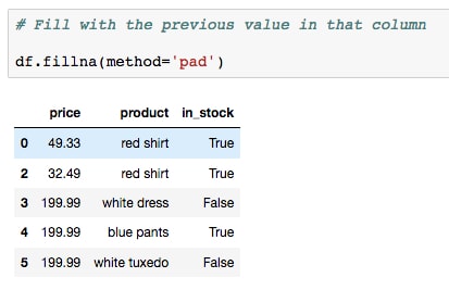
Notice how the white dress price was used to pad the missing values below it.
To conclude this section, we will prepare our simple table to be used for training a machine learning algorithm. Don't worry, we won't actually try to train any models on such a small dataset! We start this process by encoding the class labels for the categorical data.
- Before encoding the labels, run the first cell in the
Building training data setssection to add another column of data representing the average product ratings: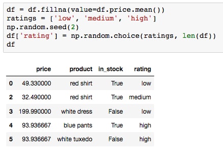
Imagining we want to use this table to train a predictive model, we should first think about changing all the variables to numeric types.
- The simplest column to handle is the Boolean list:
in_stock. This should be changed to numeric values, for example,0and1, before using it to train a predictive model. This can be done in many ways, for example, by running the cell containing the following code:df.in_stock = df.in_stock.map({False: 0, True: 1})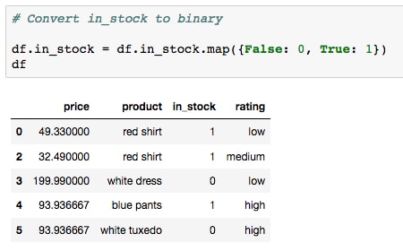
- Another option for encoding features is scikit-learn's
LabelEncoder, which can be used to map the class labels to integers at a higher level. Let's test this by running the cell containing the following code:from sklearn.preprocessing import LabelEncoder rating_encoder = LabelEncoder() _df = df.copy() _df.rating = rating_encoder.fit_transform(df.rating) _df
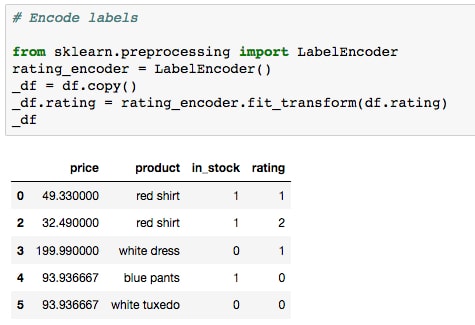
This might bring to mind the preprocessing we did in the previous lesson, when building the polynomial model. Here, we instantiate a label encoder and then "train" it and "transform" our data using the
fit_transformmethod. We apply the result to a copy of our DataFrame,_df. - The features can then be converted back using the class we reference with the variable
rating_encoder, by runningrating_encoder.inverse_transform(df.rating):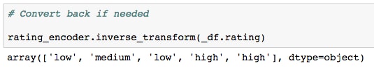
You may notice a problem here. We are working with a so-called "ordinal" feature, where there's an inherent order to the labels. In this case, we should expect that a rating of "low" would be encoded with a 0 and a rating of "high" would be encoded with a 2. However, this is not the result we see. In order to achieve proper ordinal label encoding, we should again use map, and build the dictionary ourselves.
- Encode the ordinal labels properly by running the cell containing the following code:
ordinal_map = {rating: index for index, rating in enumerate(['low', 'medium', 'high'])}
print(ordinal_map)
df.rating = df.rating.map(ordinal_map)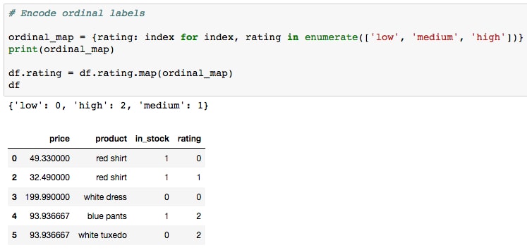
We first create the mapping dictionary. This is done using a dictionary comprehension and enumeration, but looking at the result, we see that it could just as easily be defined manually instead. Then, as done earlier for the
in_stockcolumn, we apply the dictionary mapping to the feature. Looking at the result, we see that rating now makes more sense than before, wherelowis labeled with0,mediumwith1, andhighwith2.Now that we've discussed ordinal features, let's touch on another type called nominal features. These are fields with no inherent order, and in our case, we see that
productis a perfect example.Most scikit-learn models can be trained on data like this, where we have strings instead of integer-encoded labels. In this situation, the necessary conversions are done under the hood. However, this may not be the case for all models in scikit-learn, or other machine learning and deep learning libraries. Therefore, it's good practice to encode these ourselves during preprocessing.
- A commonly used technique to convert class labels from strings to numerical values is called one-hot encoding. This splits the distinct classes out into separate features. It can be accomplished elegantly with
pd.get_dummies(). Do this by running the cell containing the following code:df = pd.get_dummies(df)
The final DataFrame then looks as follows:
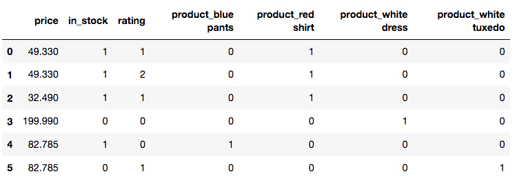
Here, we see the result of one-hot encoding: the
productcolumn has been split into 4, one for each unique value. Within each column, we find either a1or0representing whether that row contains the particular value or product.Moving on and ignoring any data scaling (which should usually be done), the final step is to split the data into training and test sets to use for machine learning. This can be done using scikit-learn's
train_test_split. Let's assume we are going to try to predict whether an item is in stock, given the other feature values. - Split the data into training and test sets by running the cell containing the following code:
features = ['price', 'rating', 'product_blue pants',
            'product_red shirt', 'product_white dress',
            'product_white tuxedo']
X = df[features].values
target = 'in_stock'
y = df[target].values
from sklearn.model_selection import train_test_split
X_train, X_test, y_train, y_test = \
    train_test_split(X, y, test_size=0.3)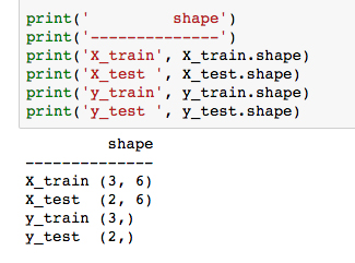
Here, we are selecting subsets of the data and feeding them into the
train_test_splitfunction. This function has four outputs, which are unpacked into the training and testing splits for features (X) and the target (y).Observe the shape of the output data, where the test set has roughly 30% of the samples and the training set has roughly 70%.
We'll see similar code blocks later, when preparing real data to use for training predictive models.
This concludes the section on cleaning data for use in machine learning applications. Let's take a minute to note how effective our Jupyter Notebook was for testing various methods of transforming the data, and ultimately documenting the pipeline we decided upon. This could easily be applied to an updated version of the data by altering only specific cells of code, prior to processing. Also, should we desire any changes to the processing, these can easily be tested in the notebook, and specific cells may be changed to accommodate the alterations. The best way to achieve this would probably be to copy the notebook over to a new file, so that we can always keep a copy of the original analysis for reference.
Moving on to an activity, we'll now apply the concepts from this section to a large dataset as we prepare it for use in training predictive models.
Suppose you are hired to do freelance work for a company who wants to find insights into why their employees are leaving. They have compiled a set of data they think will be helpful in this respect. It includes details on employee satisfaction levels, evaluations, time spent at work, department, and salary.
The company shares their data with you by sending you a file called hr_data.csv and asking what you think can be done to help stop employees from leaving.
To apply the concepts we've learned thus far to a real-life problem. In particular, we seek to:
- Determine a plan for using predictive analytics to provide impactful business insights, given the available data.
- Prepare the data for use in machine learning models.
Note
Starting with this activity and continuing through the remainder of this lesson, we'll be using Human Resources Analytics, which is a Kaggle dataset.
There is a small difference between the dataset we use in this book and the online version. Our human resource analytics data contains some NaN values. These were manually removed from the online version of the dataset, for the purposes of illustrating data cleaning techniques. We have also added a column of data called is_smoker, for the same purposes.
- With the
lesson-2-workbook.ipynbnotebook file open, scroll to theActivity Asection. - Check the head of the table by running the following code:
%%bash
head ../data/hr-analytics/hr_data.csv
Judging by the output, convince yourself that it looks to be in standard CSV format. For CSV files, we should be able to simply load the data with
pd.read_csv. - Load the data with Pandas by running
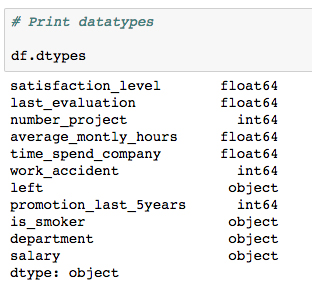
df = pd.read_csv('../data/hr-analytics/hr_data.csv'). Use tab completion to help type the file path. - Inspect the columns by printing
df.columnsand make sure the data has loaded as expected by printing the DataFrameheadandtailwithdf.head()anddf.tail():
We can see that it appears to have loaded correctly. Based on the
tailindex values, there are nearly 15,000 rows; let's make sure we didn't miss any. - Check the number of rows (including the header) in the CSV file with the following code:
with open('../data/hr-analytics/hr_data.csv') as f:
    print(len(f.read().splitlines()))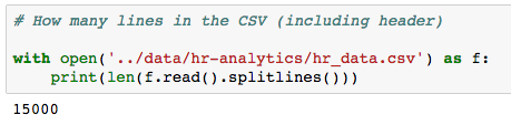
- Compare this result to
len(df)to make sure we've loaded all the data: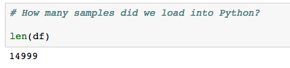
Now that our client's data has been properly loaded, let's think about how we can use predictive analytics to find insights into why their employees are leaving.
Let's run through the first steps for creating a predictive analytics plan:
- Look at the available data: We've already done this by looking at the columns, datatypes, and the number of samples
- Determine the business needs: The client has clearly expressed their needs: reduce the number of employees who leave
- Assess the data for suitability: Let's try to determine a plan that can help satisfy the client's needs, given the provided data
Recall, as mentioned earlier, that effective analytics techniques lead to impactful business decisions. With that in mind, if we were able to predict how likely an employee is to quit, the business could selectively target those employees for special treatment. For example, their salary could be raised or their number of projects reduced. Furthermore, the impact of these changes could be estimated using the model!
To assess the validity of this plan, let's think about our data. Each row represents an employee who either works for the company or has left, as labeled by the column named left. We can therefore train a model to predict this target, given a set of features.
Assess the target variable. Check the distribution and number of missing entries by running the following code:
df.left.value_counts().plot('barh')
print(df.left.isnull().sum())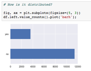
Here's the output of the second code line:
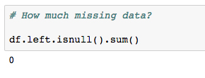
About three-quarters of the samples are employees who have not left. The group who has left makes up the other quarter of the samples. This tells us we are dealing with an imbalanced classification problem, which means we'll have to take special measures to account for each class when calculating accuracies. We also see that none of the target variables are missing (no NaN values).
Now, we'll assess the features:
This code snippet is a little complicated, but it's very useful for showing an overview of both the continuous and discrete features in our dataset. Essentially, it assumes each feature is continuous and attempts to plot its distribution, and reverts to simply plotting the value counts if the feature turns out to be discrete.
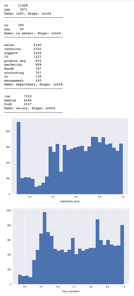
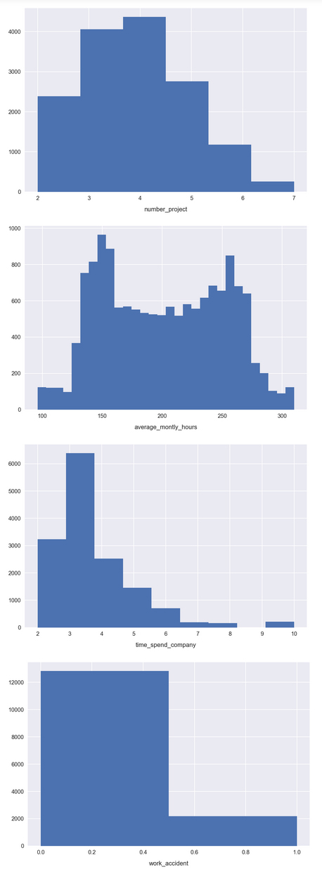
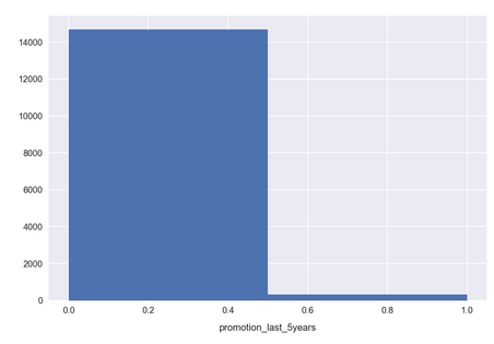
For many features, we see a wide distribution over the possible values, indicating a good variety in the feature spaces. This is encouraging; features that are strongly grouped around a small range of values may not be very informative for the model. This is the case for promotion_last_5years, where we see that the vast majority of samples are 0.
The next thing we need to do is remove any NaN values from the dataset.
- Check how many
NaNvalues are in each column by running the following code:df.isnull().sum() / len(df) * 100
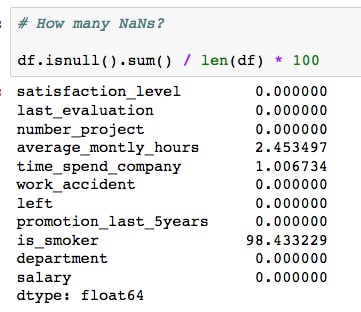
We can see there are about 2.5% missing for
average_montly_hours, 1% missing fortime_spend_company, and 98% missing foris_smoker! Let's use a couple of different strategies that we've learned about to handle these. - Since there is barely any information in the
is_smokermetric, let's drop this column. Do this by running:del df['is_smoker']. - Since
time_spend_companyis an integer field, we'll use the median value to fill theNaNvalues in this column. This can be done with the following code:fill_value = df.time_spend_company.median() df.time_spend_company = df.time_spend_company.fillna(fill_value)
The final column to deal with is
average_montly_hours. We could do something similar and use the median or rounded mean as the integer fill value. Instead though, let's try to take advantage of its relationship with another variable. This may allow us to fill the missing data more accurately. - Make a boxplot of
average_montly_hourssegmented bynumber_project. This can be done by running the following code:sns.boxplot(x='number_project', y='average_montly_hours', data=df)
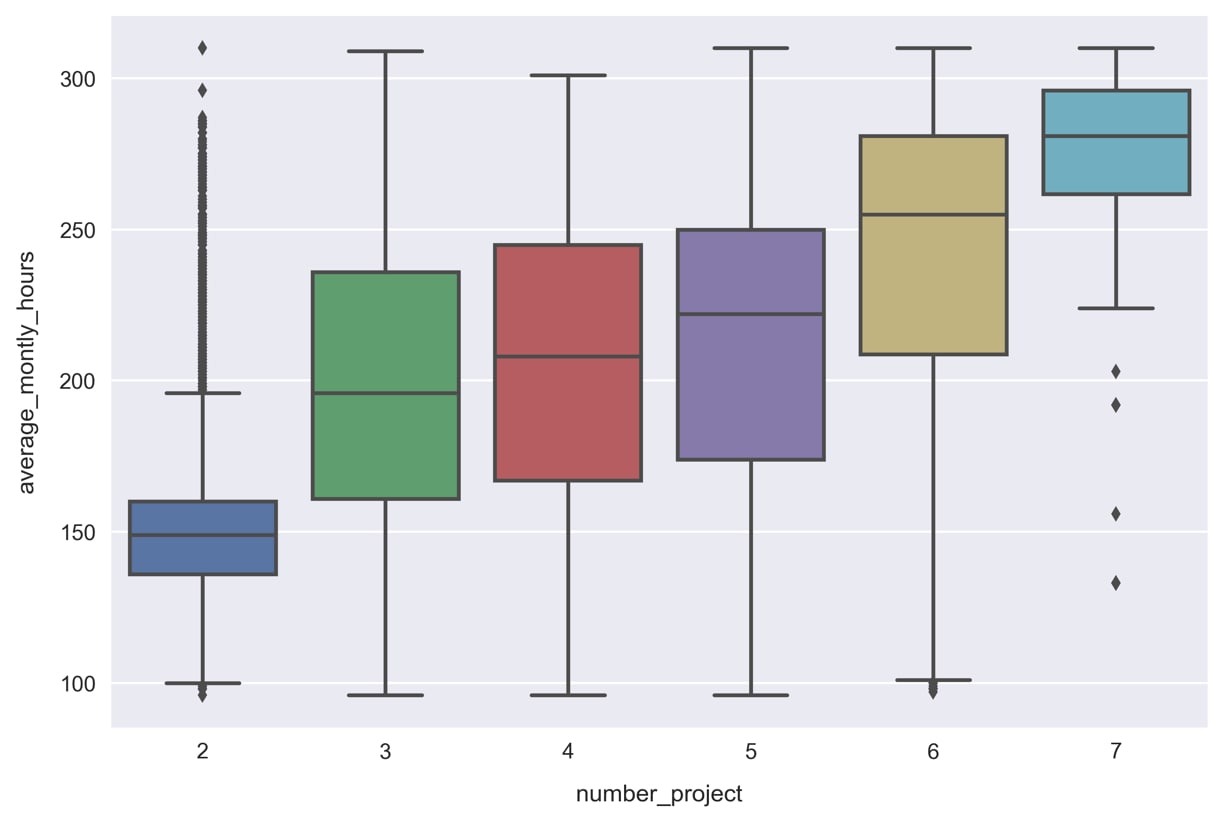
We can see how the number of projects is correlated with
average_monthly_hours, a result that is hardly surprising. We'll exploit this relationship by filling in theNaNvalues ofaverage_montly_hoursdifferently, depending on the number of projects for that sample. Specifically, we'll use the mean of each group. - Calculate the mean of each group by running the following code:
mean_per_project = df.groupby('number_project')\
                    .average_montly_hours.mean()
mean_per_project = dict(mean_per_project)
print(mean_per_project)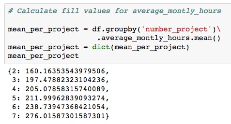
We can then map this onto the
number_projectcolumn and pass the resulting series object as the argument tofillna. - Fill the
NaNvalues inaverage_montly_hoursby executing the following code:fill_values = df.number_project.map(mean_per_project) df.average_montly_hours = df.average_montly_hours.fillna(fill_values)
- Confirm that
dfhas no moreNaNvalues by running the following assertion test. If it does not raise an error, then you have successfully removed theNaNs from the table:assert df.isnull().sum().sum() == 0
- Finally, we will transform the string and Boolean fields into integer representations. In particular, we'll manually convert the target variable
leftfromyesandnoto1and0and build the one-hot encoded features. Do this by running the following code:df.left = df.left.map({'no': 0, 'yes': 1}) df = pd.get_dummies(df) - Print
df.columnsto show the fields:
We can see that
departmentandsalaryhave been split into various binary features.The final step to prepare our data for machine learning is scaling the features, but for various reasons (for example, some models do not require scaling), we'll do it as part of the model-training workflow in the next activity.
- We have completed the data preprocessing and are ready to move on to training models! Let's save our preprocessed data by running the following code:
df.to_csv('../data/hr-analytics/hr_data_processed.csv', index=False)
Again, we pause here to note how well the Jupyter Notebook suited our needs when performing this initial data analysis and clean-up. Imagine, for example, we left this project in its current state for a few months. Upon returning to it, we would probably not remember what exactly was going on when we left it. Referring back to this notebook though, we would be able to retrace our steps and quickly recall what we previously learned about the data. Furthermore, we could update the data source with any new data and re-run the notebook to prepare the new set of data for use in our machine learning algorithms. Recall that in this situation, it would be best to make a copy of the notebook first, so as not to lose the initial analysis.
To summarize, we've learned and applied methods for preparing to train a machine learning model. We started by discussing steps for identifying a problem that can be solved with predictive analytics. This consisted of:
- Looking at the available data
- Determining the business needs
- Assessing the data for suitability
We also discussed how to identify supervised versus unsupervised and regression versus classification problems.
After identifying our problem, we learned techniques for using Jupyter Notebooks to build and test a data transformation pipeline. These techniques included methods and best practices for filling missing data, transforming categorical features, and building train/test data sets.
In the remainder of this lesson, we will use this preprocessed data to train a variety of classification models. To avoid blindly applying algorithms we don't understand, we start by introducing them and overviewing how they work. Then, we use Jupyter to train and compare their predictive capabilities. Here, we have the opportunity to discuss more advanced topics in machine learning like overfitting, k-fold cross-validation, and validation curves.