Scraping Web Page Data

In the spirit of leveraging the internet as a database, we can think about acquiring data from web pages either by scraping content or by interfacing with web APIs. Generally, scraping content means getting the computer to read data that was intended to be displayed in a human-readable format. This is in contradistinction to web APIs, where data is delivered in machine-readable formats – the most common being JSON.

In this topic, we will focus on web scraping. The exact process for doing this will depend on the page and desired content. However, as we will see, it's quite easy to scrape anything we need from an HTML page so long as we have an understanding of the underlying concepts and tools. In this topic, we'll use Wikipedia as an example and scrape tabular content from an article. Then, we'll apply the same techniques to scrape data from a page on an entirely separate domain. But first, we'll take some time to introduce HTTP requests.

Subtopic A: Introduction to HTTP Requests

The Hypertext Transfer Protocol, or HTTP for short, is the foundation of data communication for the internet. It defines how a page should be requested and how the response should look. For example, a client can request an Amazon page of laptops for sale, a Google search of local restaurants, or their Facebook feed. Along with the URL, the request will contain the user agent and available browsing cookies among the contents of the request header. The user agent tells the server what browser and device the client is using, which is usually used to provide the most user-friendly version of the web page's response. Perhaps they have recently logged in to the web page; such information would be stored in a cookie that might be used to automatically log the user in.

These details of HTTP requests and responses are taken care of under the hood thanks to web browsers. Luckily for us, today the same is true when making requests with high-level languages such as Python. For many purposes, the contents of request headers can be largely ignored. Unless otherwise specified, these are automatically generated in Python when requesting a URL. Still, for the purposes of troubleshooting and understanding the responses yielded by our requests, it's useful to have a foundational understanding of HTTP.

There are many types of HTTP methods, such as GET, HEAD, POST, and PUT. The first two are used for requesting that data be sent from the server to the client, whereas the last two are used for sending data to the server.

These HTTP methods are summarized in the following table:

HTTP method	Description
GET	Retrieves the information from the specified URL
HEAD	Retrieves the meta information from the HTTP header of the specified URL
POST	Sends the attached information for appending to the resource(s) at the specified URL
PUT	Sends the attached information for replacing the resource(s) at the specified URL

A GET request is sent each time we type a web page address into our browser and press Enter. For web scraping, this is usually the only HTTP method we are interested in, and it's the only method we'll be using in this lesson.

Once the request has been sent, a variety of response types can be returned from the server. These are labeled with 100-level to 500-level codes, where the first digit in the code represents the response class. These can be described as follows:

1xx: Informational response, for example, server is processing a request. It's uncommon to see this.
2xx: Success, for example, page has loaded properly.
3xx: Redirection, for example, the requested resource has been moved and we were redirected to a new URL.
4xx: Client error, for example, the requested resource does not exist.
5xx: Server error, for example, the website server is receiving too much traffic and could not fulfill the request.

For the purposes of web scraping, we usually only care about the response class, that is, the first digit of the response code. However, there exist subcategories of responses within each class that offer more granularity on what's going on. For example, a 401 code indicates an unauthorized response, whereas a 404 code indicates a page not found response. This distinction is noteworthy because a 404 would indicate we've requested a page that does not exist, whereas 401 tells us we need to log in to view the particular resource.

Let's see how HTTP requests can be done in Python and explore some of these topics using the Jupyter Notebook.

Subtopic B: Making HTTP Requests in the Jupyter Notebook

Now that we've talked about how HTTP requests work and what type of responses we should expect, let's see how this can be done in Python. We'll use a library called Requests, which happens to be the most downloaded external library for Python. It's possible to use Python's built-in tools, such as urllib, for making HTTP requests, but Requests is far more intuitive, and in fact it's recommended over urllib in the official Python documentation.

Requests is a great choice for making simple and advanced web requests. It allows for all sorts of customization with respect to headers, cookies, and authorization. It tracks redirects and provides methods for returning specific page content such as JSON. Furthermore, there's an extensive suite of advanced features. However, it does not allow JavaScript to be rendered.

Note

Oftentimes, servers return HTML with JavaScript code snippets included, which are automatically run in the browser on load time. When requesting content with Python using Requests, this JavaScript code is visible, but it does not run. Therefore, any elements that would be altered or created by doing so are missing. Often, this does not affect the ability to get the desired information, but in some cases we may need to render the JavaScript in order to scrape the page properly. For doing this, we could use a library like Selenium. This has a similar API to the Requests library, but provides support for rendering JavaScript using web drivers.

Let's dive into the following section using the Requests library with Python in a Jupyter Notebook.

Handling HTTP requests with Python in a Jupyter Notebook

Start the NotebookApp from the project directory by executing jupyter notebook. Navigate to the lesson-3 directory and open up the lesson-3-workbook.ipynb file. Find the cell near the top where the packages are loaded and run it.
We are going to request a web page and then examine the response object. There are many different libraries for making requests and many choices for exactly how to do so with each. We'll only use the Requests library, as it provides excellent documentation, advanced features, and a simple API.
Scroll down to Subtopic A: Introduction to HTTP requests and run the first cell in that section to import the Requests library. Then, prepare a request by running the cell containing the following code:
```
url = 'https://jupyter.org/'
req = requests.Request('GET', url)
req.headers['User-Agent'] = 'Mozilla/5.0'
req = req.prepare()
```
We use the Request class to prepare a GET request to the jupyter.org homepage. By specifying the user agent as Mozilla/5.0, we are asking for a response that would be suitable for a standard desktop browser. Finally, we prepare the request.
Print the docstring for the "prepared request" req, by running the cell containing req?: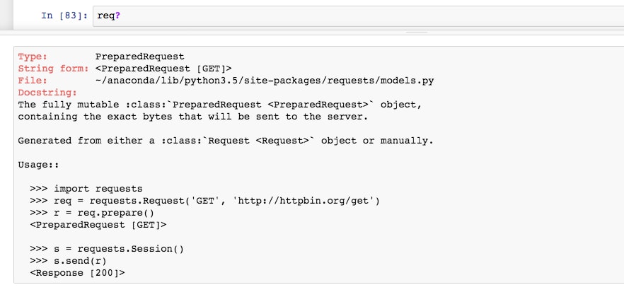
Looking at its usage, we see how the request can be sent using a session. This is similar to opening a web browser (starting a session) and then requesting a URL.
Make
the request and store the response in a variable named page, by running the following code:
```
with requests.Session() as sess:
    page = sess.send(req)
```
This code returns the HTTP response, as referenced by the page variable. By using the with statement, we initialize a session whose scope is limited to the indented code block. This means we do not have to worry about explicitly closing the session, as it is done automatically.
Run the next two cells in the notebook to investigate the response. The string representation of page should indicate a 200 status code response. This should agree with the status_code attribute.
Save the response text to the page_html variable and take a look at the head of the string with page_html[:1000]: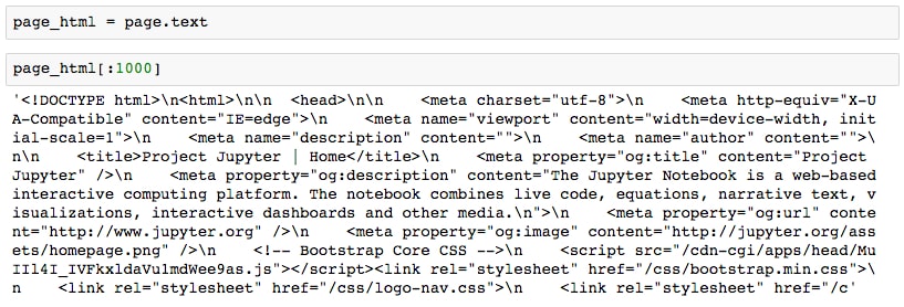
As expected, the response is HTML. We can format this output better with the help of BeautifulSoup, a library which will be used extensively for HTML parsing later in this section.
Print
the head of the formatted HTML by running the following:
```
from bs4 import BeautifulSoup
print(BeautifulSoup(page_html, 'html.parser').prettify()[:1000])
```
We import BeautifulSoup and then print the pretty output, where newlines are indented depending on their hierarchy in the HTML structure.
We can take this a step further and actually display the HTML in Jupyter by using the IPython display module. Do this by running the following code:
```
from IPython.display import HTML
HTML(page_html)
```
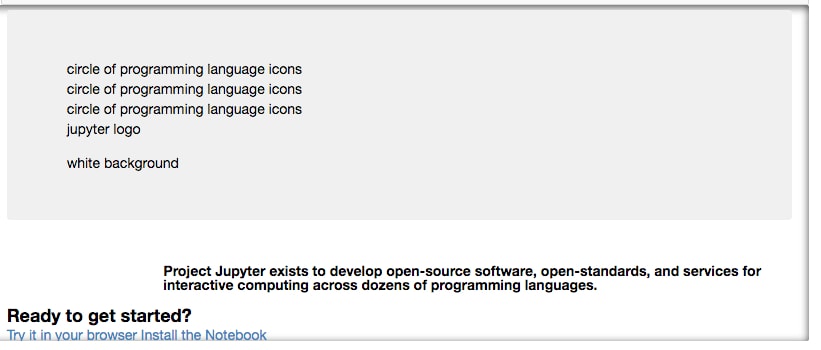
Here, we see the HTML rendered as well as possible, given that no JavaScript code has been run and no external resources have loaded. For example, the images that are hosted on the jupyter.org server are not rendered and we instead see the alt text: circle of programming icons, jupyter logo, and so on.
Let's compare this to the live website, which can be opened in Jupyter using an IFrame. Do this by running the following code:
```
from IPython.display import IFrame
IFrame(src=url, height=800, width=800)
```
Here, we see the full site rendered, including JavaScript and external resources. In fact, we can even click on the hyperlinks and load those pages in the IFrame, just like a regular browsing session.
It's good practice to close the IFrame after using it. This prevents it from eating up memory and processing power. It can be closed by selecting the cell and clicking Current Outputs | Clear from the Cell menu in the Jupyter Notebook.
Recall how we used a prepared request and session to request this content as a string in Python. This is often done using a shorthand method instead. The drawback is that we do not have as much customization of the request header, but that's usually fine.
Make a request to http://www.python.org/ by running the following code:
```
url = 'http://www.python.org/'page = requests.get(url)
page
<Response [200]>
```
The string representation of the page (as displayed beneath the cell) should indicate a 200 status code, indicating a successful response.
Run the next two cells. Here, we print the url and history attributes of our page.
The URL returned is not what we input; notice the difference? We were redirected from the input URL, http://www.python.org/, to the secured version of that page, https://www.python.org/. The difference is indicated by an additional s at the start of the URL, in the protocol. Any redirects are stored in the history attribute; in this case, we find one page in here with status code 301 (permanent redirect), corresponding to the original URL requested.

Now that we're comfortable making requests, we'll turn our attention to parsing the HTML. This can be something of an art, as there are usually multiple ways to approach it, and the best method often depends on the details of the specific HTML in question.

Subtopic C: Parsing HTML in the Jupyter Notebook

When scraping data from a web page, after making the request, we must extract the data from the response content. If the content is HTML, then the easiest way to do this is with a high-level parsing library such as Beautiful Soup. This is not to say it's the only way; in principle, it would be possible to pick out the data using regular expressions or Python string methods such as split, but pursuing either of these options would be an inefficient use of time and could easily lead to errors. Therefore, it's generally frowned upon and instead, the use of a trustworthy parsing tool is recommended.

In order to understand how content can be extracted from HTML, it's important to know the fundamentals of HTML. For starters, HTML stands for Hyper Text Markup Language. Like Markdown or XML (eXtensible Markup Language), it's simply a language for marking up text. In HTML, the display text is contained within the content section of HTML elements, where element attributes specify how that element should appear on the page.

Subtopic C: Parsing HTML in the Jupyter Notebook

Looking at the anatomy of an HTML element, as seen in the preceding picture, we see the content enclosed between start and end tags. In this example, the tags are <p> for paragraph; other common tag types are <div> (text block), <table> (data table), <h1> (heading), <img> (image), and <a> (hyperlinks). Tags have attributes, which can hold important metadata. Most commonly, this metadata is used to specify how the element text should appear on the page. This is where CSS files come into play. The attributes can store other useful information, such as the hyperlink href in an <a> tag, which specifies a URL link, or the alternate alt label in an <img> tag, which specifies the text to display if the image resource cannot be loaded.

Now, let's turn our attention back to the Jupyter Notebook and parse some HTML! Although not necessary when following along with this section, it's very helpful in real-world situations to use the developer tools in Chrome or Firefox to help identify the HTML elements of interest. We'll include instructions for doing this with Chrome in the following section.

Parsing HTML with Python in a Jupyter Notebook

In lesson-3-workbook.ipynb file, scroll to the top of Subtopic B: Parsing HTML with Python.
In this section, we'll scrape the central bank interest rates for each country, as reported by Wikipedia. Before diving into the code, let's first open up the web page containing this data.
Open up the https://en.wikipedia.org/wiki/List_of_countries_by_central_bank_interest_rates URL in a web browser. Use Chrome, if possible, as later in this section we'll show you how to view and search the HTML with Chrome's developer tools.
Looking at the page, we see very little content other than a big list of countries and their interest rates. This is the table we'll be scraping.
Return to the Jupyter Notebook and load the HTML as a Beautiful Soup object so that it can be parsed. Do this by running the following code:
```
from bs4 import BeautifulSoup
soup = BeautifulSoup(page.content, 'html.parser')
```
We use Python's default html.parser as the parser, but third-party parsers such as lxml may be used instead, if desired.
Usually, when working with a new object like this Beautiful Soup one, it's a good idea to pull up the docstring by doing soup?. However, in this case, the docstring is not particularly informative. Another tool for exploring Python objects is pdir, which lists all of an object's attributes and methods (this can be installed with pip install pdir2). It's basically a formatted version of Python's built-in dir function.
Display the attributes and methods for the BeautifulSoup object
by running the following code. This will run, regardless of whether or not the pdir external library is installed:
```
try:import pdirdir = pdir
except:
    print('You can install pdir with:\npip install pdir2')
dir(soup)
```
Here, we see a list of methods and attributes that can be called on soup. The most commonly used function is probably find_all, which returns a list of elements that match the given criteria.
Get the h1 heading for the page with the following code:
```
h1 = soup.find_all('h1')
h1
>> [<h1 class="firstHeading" id="firstHeading" lang="en">List of countries by central bank interest rates</h1>]
```
Usually, pages only have one H1 element, so it's obvious that we only find one here.
Run the next couple of cells. We redefine H1 to the first (and only) list element with h1 = h1[0], and then print out the HTML element attributes with h1.attrs:
```
>> {'class': ['firstHeading'], 'id': 'firstHeading', 'lang': 'en'}
```
We see the class and ID of this element, which can both be referenced by CSS code to define the style of this element.
Get the HTML element content (that is, the visible text) by printing h1.text.
Get
all the images on the page by running the following code:
```
imgs = soup.find_all('img')
len(imgs)
>> 91
```
There are lots of images on the page. Most of these are for the country flags.
Print the source of each image by running the following code:
```
[element.attrs['src'] for element in imgsif 'src' in element.attrs.keys()]
```
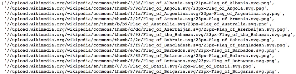
We use a list comprehension to iterate through the elements, selecting the src attribute of each (so long as that attribute is actually available).
Now, let's scrape the table. We'll use Chrome's developer tools to hunt down the element this is contained within.
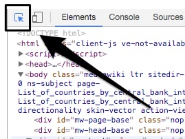
If not already done, open the Wikipedia page we're looking at in Chrome. Then, in the browser, select Developer Tools from the View menu. A sidebar will open. The HTML is available to look at from the Elements tab in Developer Tools.
Select the little arrow in the top left of the tools sidebar. This allows us to hover over the page and see where the HTML element is located, in the Elements section of the sidebar:
Hover over the body to see how the table is contained within the div that has id="bodyContent":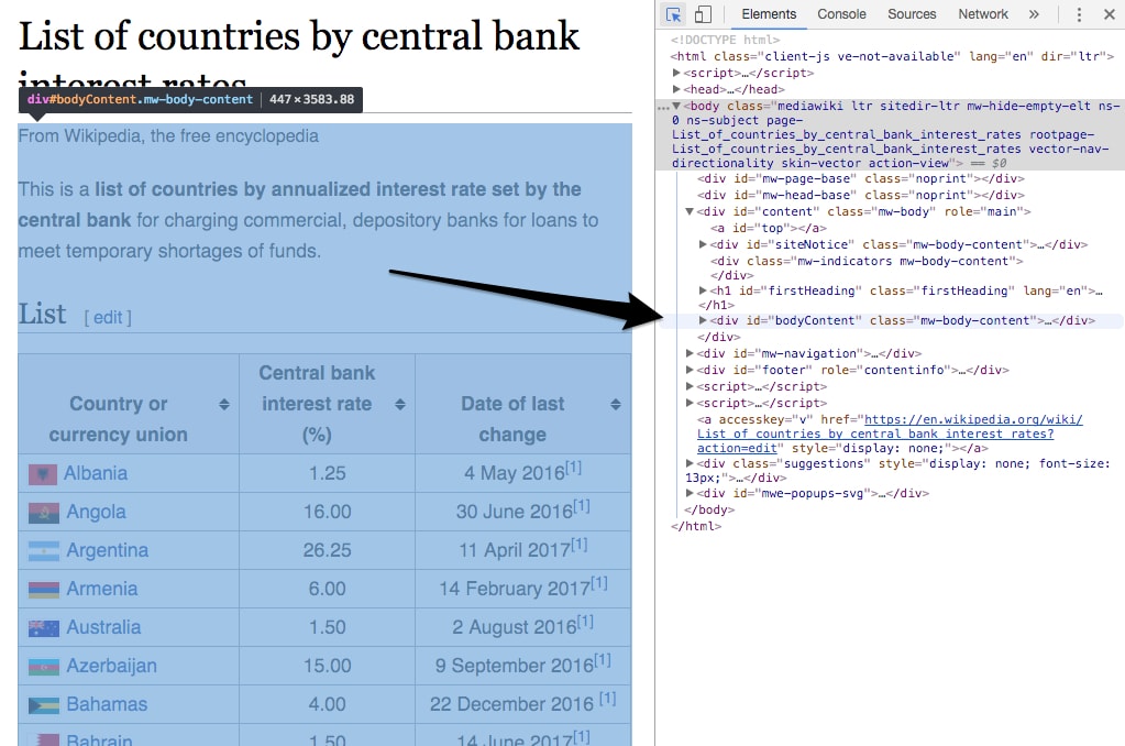
Select
that div by running the following code:
```
body_content = soup.find('div', {'id': 'bodyContent'})
```
We can now seek out the table within this subset of the full HTML. Usually, tables are organized into headers <th>, rows <tr>, and data entries <td>.

Get the table headers by running the following code:

table_headers = body_content.find_all('th')[:3]table_headers
>>> [<th>Country or<br/>
     currency union</th>, <th>Central bank<br/>
     interest rate (%)</th>, <th>Date of last<br/>
     change</th>]

Here, we see three headers. In the content of each is a break element <br/>, which will make the text a bit more difficult to cleanly parse.

Get
the text by running the following code:
```
table_headers = [element.get_text().replace('\n', ' ')for element in table_headers]table_headers
 >> ['Country or currency union',
    'Central bank interest rate (%)',
    'Date of last change']
```
Here, we get the content with the get_text method, and then run the replace string method to remove the newline resulting from the <br/> element.
To get the data, we'll first perform some tests and then scrape all the data in a single cell.
Get the data for each cell in the second <tr> (row) element by running the following code:
```
row_number = 2d1, d2, d3 = body_content.find_all('tr')[row_number]\.find_all('td')
```
We find all the row elements, pick out the third one, and then find the three data elements inside that.
Let's look at the resulting data and see how to parse the text from each row.
Run the next couple of cells to print d1 and its text attribute: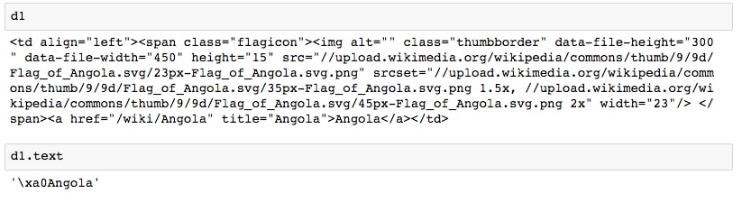
We're getting some undesirable characters at the front. This can be solved by searching for only the text of the <a> tag.
Run d1.find('a').text to return the properly cleaned data for that cell.
Run the next couple of cells to print d2 and its text. This data appears to be clean enough to convert directly into a float.
Run the next couple of cells to print d3 and its text: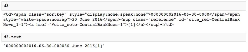
Similar to d1, we see that it would be better to get only the span element's text.
Properly parse the date for this table entry by running the following code:
```
d3.find_all('span')[1].text
>> '30 June 2016'
```
Now, we're ready to perform the full scrape by iterating over the row elements <th>. Run the following code:
```
data = []for i, row in enumerate(body_content.find_all('tr')):...
...
>> Ignoring row 101 because len(data) != 3
>> Ignoring row 102 because len(data) != 3
```
Note
For the complete code, refer to the Lesson 3.txt file in the Lesson 3 folder.
We iterate over the rows, ignoring any that contain more than three data elements. These rows will not correspond to data in the table we are interested in. Rows that do have three data elements are assumed to be in the table, and we parse the text from these as identified during the testing.
The text parsing is done inside a try/except statement, which will catch any errors and allow this row to be skipped without stopping the iteration. Any rows that raise errors due to this statement should be looked at. The data for these could be recorded manually or accounted for by altering the scraping loop and re-running it. In this case, we'll ignore any errors for the sake of time.

Print the head of the scraped data list by running print(data[:10]):

>> [['Albania', 1.25, '4 May 2016'],
    ['Angola', 16.0, '30 June 2016'],
    ['Argentina', 26.25, '11 April 2017'],
    ['Armenia', 6.0, '14 February 2017'],
    ['Australia', 1.5, '2 August 2016'],
    ['Azerbaijan', 15.0, '9 September 2016'],
    ['Bahamas', 4.0, '22 December 2016'],
    ['Bahrain', 1.5, '14 June 2017'],
    ['Bangladesh', 6.75, '14 January 2016'],
    ['Belarus', 12.0, '28 June 2017']]

We'll visualize this data later in the lesson. For now, save the data to a CSV file by running the following code:

f_path = '../data/countries/interest-rates.csv'with open(f_path, 'w') as f:f.write('{};{};{}\n'.format(*table_headers))for d in data:f.write('{};{};{}\n'.format(*d))

Note that we are using semicolons to separate the fields.

Activity A: Web Scraping with Jupyter Notebooks

We are going to get the population of each country. Then, in the next topic, this will be visualized along with the interest rate data scraped in the previous section.

The page we look at in this activity is available here: http://www.worldometers.info/world-population/population-by-country/.

Now that we've seen the basics of web scraping, let's apply the same techniques to a new web page and scrape some more data!

Note

This page may have changed since this document was created. If this URL no longer leads to a table of country populations, please use this Wikipedia page instead: https://en.wikipedia.org/wiki/List_of_countries_by_population (United_Nations).

For this page, the data can be scraped using the following code snippet:

data = []
for i, row in enumerate(soup.find_all('tr')):
	row_data = row.find_all('td')
	try:
		d1, d2, d3 = row_data[1], row_data[5], row_data[6]
		d1 = d1.find('a').text
		d2 = float(d2.text)
		d3 = d3.find_all('span')[1].text.replace('+', '')
		data.append([d1, d2, d3])
except:
		print('Ignoring row {}'.format(i))

In the lesson-3-workbook.ipynb Jupyter Notebook, scroll to Activity A: Web scraping with Python.
Set the url variable and load an IFrame of our page in the notebook by running the following code:
```
url = 'http://www.worldometers.info/world-population/population-by-country/'
IFrame(url, height=300, width=800)
```
The page should load in the notebook. Scrolling down, we can see the Countries in the world by population heading and the table of values beneath it. We'll scrape the first three columns from this table to get the countries, populations, and yearly population changes.
Close the IFrame by selecting the cell and clicking Current Outputs | Clear from the Cell menu in the Jupyter Notebook.
Request the page and load it as a BeautifulSoup object by running the following code:
```
page = requests.get(url)soup = BeautifulSoup(page.content, 'html.parser')
```
We feed the page content to the BeautifulSoup constructor. Recall that previously, we used page.text here instead. The difference is that page.content returns the raw binary response content, whereas page.text returns the UTF-8 decoded content. It's usually best practice to pass the bytes object and let BeautifulSoup decode it, rather than doing it with Requests using page.text.
Print the H1 for the page by running the following code:
```
soup.find_all('h1')
>> [<h1>Countries in the world by population (2017)</h1>]
```
We'll scrape the table by searching for <th>, <tr>, and <td> elements, as in the previous section.

Get and print the table headings by running the following code:

table_headers = soup.find_all('th')table_headers
>> [<th>#</th>,
   <th>Country (or dependency)</th>,
   <th>Population<br/> (2017)</th>,
   <th>Yearly<br/> Change</th>,
   <th>Net<br/> Change</th>,
   <th>Density<br/> (P/Km²)</th>,
   <th>Land Area<br/> (Km²)</th>,
   <th>Migrants<br/> (net)</th>,
   <th>Fert.<br/> Rate</th>,
   <th>Med.<br/> Age</th>,
   <th>Urban<br/> Pop %</th>,
   <th>World<br/> Share</th>]

We are only interested in the first three columns. Select these and parse the text with the
following code:
```
table_headers = table_headers[1:4]
table_headers = [t.text.replace('\n', '') for t in table_headers]
```
After selecting the subset of table headers we want, we parse the text content from each and remove any newline characters.
Now, we'll get the data. Following the same prescription as the previous section, we'll test how to parse the data for a sample row.

Get the data for a sample row by running the following code:

row_number = 2row_data = soup.find_all('tr')[row_number]\
                .find_all('td')

How many columns of data do we have? Print the length of row_data by running print(len(row_data)).

Print the first elements by running print(row_data[:4]):

>> [<td>2</td>,
   <td style="font-weight: bold; font-size:15px; text-align:left"><a href="/world-population/india-population/">India</a></td>,
   <td style="font-weight: bold;">1,339,180,127</td>,
   <td>1.13 %</td>]

It's pretty obvious that we want to select list indices 1, 2, and 3. The first data value can be ignored, as it's simply the index.

Select the data elements we're interested in parsing by running the following code:
```
d1, d2, d3 = row_data[1:4]
```
Looking at the row_data output, we can find out how to correctly parse the data. We'll want to select the content of the <a> element in the first data element, and then simply get the text from the others. Test these assumptions by running the following code:
```
print(d1.find('a').text)print(d2.text)print(d3.text)
>> India
>> 1,339,180,127
>> 1.13 %
```
Excellent! This looks to be working well. Now, we're ready to scrape the entire table.

Scrape and parse the table data by running the following code:

data = []for i, row in enumerate(soup.find_all('tr')):try:d1, d2, d3 = row.find_all('td')[1:4]d1 = d1.find('a').textd2 = d2.textd3 = d3.textdata.append([d1, d2, d3])except:print('Error parsing row {}'.format(i))
>> Error parsing row 0

This is quite similar to before, where we try to parse the text and skip the row if there's some error.

Print the head of the scraped data by running print(data[:10]):

>> [['China', '1,409,517,397', '0.43 %'],
   ['India', '1,339,180,127', '1.13 %'],
   ['U.S.', '324,459,463', '0.71 %'],
   ['Indonesia', '263,991,379', '1.10 %'],
   ['Brazil', '209,288,278', '0.79 %'],
   ['Pakistan', '197,015,955', '1.97 %'],
   ['Nigeria', '190,886,311', '2.63 %'],
   ['Bangladesh', '164,669,751', '1.05 %'],
   ['Russia', '143,989,754', '0.02 %'],
   ['Mexico', '129,163,276', '1.27 %']]

It looks like we have managed to scrape the data! Notice how similar the process was for this table compared to the Wikipedia one, even though this web page is completely different. Of course, it will not always be the case that data is contained within a table, but regardless, we can usually use find_all as the primary method for parsing.

Finally, save the data to a CSV file for later use. Do this by running the following code:

f_path = '../data/countries/populations.csv'with open(f_path, 'w') as f:f.write('{};{};{}\n'.format(*table_headers))for d in data:
        f.write('{};{};{}\n'.format(*d))

To summarize, we've seen how Jupyter Notebooks can be used for web scraping. We started this lesson by learning about HTTP methods and status codes. Then, we used the Requests library to actually perform HTTP requests with Python and saw how the Beautiful Soup library can be used to parse the HTML responses.

Our Jupyter Notebook turned out to be a great tool for this type of work. We were able to explore the results of our web requests and experiment with various HTML parsing techniques. We were also able to render the HTML and even load a live version of the web page inside the notebook!

In the next topic of this lesson, we shift to a completely new topic: interactive visualizations. We'll see how to create and display interactive charts right inside the notebook, and use these charts as a way to explore the data we've just collected.