Chapter 20
Mortgage Default Modeling
Worm or beetle—drought or tempest—on a farmer's land may fall, each is loaded full o' ruin, but a mortgage beats em' all.
–Will Carleton
Up to this point, the focus of this book has been the evaluation of securities whose credit enhancement is external to the structure. The most common and well known is the corporate guarantee of the government-sponsored enterprises Fannie Mae (FNMA), Freddie Mac (FHLMC), and the Government National Mortgage Association (GNMA). Only GNMA securities carry the full faith and credit pledge of the U.S. government—an explicit guarantee. Both FNMA's and FHLMC's guarantees are corporate. However, the U.S. government acts as a credit backstop, and both FNMA and FHLMC securities are said to carry an implicit government guarantee.1
MBS structures that rely on an internal credit enhancement mechanism are self-insuring and are often referred to as private-label MBS (PLMBS) or non-agency MBS. The terms private-label and non-agency MBS are used to differentiate those MBS transactions whose credit enhancement is internally created from those whose credit enhancement relies on either a direct or indirect government guarantee.
A mortgage default arises from the following:
- Poor underwriting standards are used.
- The borrower experiences a life event such as:
- Long-term unemployment
- Illness or disability
- Family break-up
- Home prices decline precipitously and the borrower finds himself in a negative equity position, leading to a strategic default.
Modeling the mortgage default rate will follow the general framework of modeling of voluntary prepayment rates. However, in this case we will employ logistic regression analysis—a parametric modeling technique rather than the proportional hazards approached outlined in Chapter 8. Other potential modeling strategies include:
- Cox proportional hazards model
- Competing risks proportional hazard model
- Multinomial logistic regression model
Both the competing risks and multinomial models are usually designed to include delinquency transition rates as a predictor in the default model, a topic addressed later in this chapter. To begin the analysis of mortgage default (involuntary prepayment) a survival function is used to extract the hazard rate and translate it to a default curve—event code 2 in the data set. Figures 20.1 and 20.2 present the cumulative survival rate and its translation to the conditional default rate CDR. In aggregate, the conditional default rate begins at 0.0 CDR in the first month and increases to around 2.5 CDR by month 48. The CDR remains at or above 2.5 through month 60, after which the CDR begins to gradually decline. Thereafter, the conditional default rate stabilizes around 1.5 CDR.
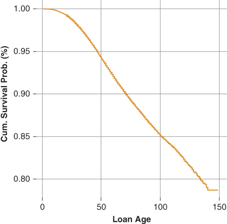
Figure 20.1 FH 30-yr. Cum. Survival

Figure 20.2 FH 30-yr. CDR
The standard default rate assumption SDA curve used to value both agency and prime credit borrower private-label mortgage-backed securities assumes the default rate begins at 0.02 CDR in the first month and increases linearly by 0.02 CDR up to month 30, where it reaches its maximum value of 0.60 CDR. Thereafter, the SDA curve assumes a flat default rate through month 60, after which it declines linearly to a minimum of 0.03 CDR per month.
20.1 Case Study FHLMC 30-Year Default Analysis
This case study uses FHLMC's sample loan level data set as of August 2013. The sample data set contains contains 50,000 loans randomly selected from each full vintage year from 2000 through 2011 and a proportionate share of loans from each partial vintage year 1999 and 2012. In all, the data set used for this case included 675,000 loans originated between January 1999 and July 2012.
The updated loan-to-value ratio is calculated using the Federal Housing Finance Agency (FHFA) state home price index. To measure home price appreciation and therefore updated LTV, each loan is referenced to the home price index value reported in the quarter corresponding to its origination date. This becomes the loan's base home price index value. The home price is updated quarterly based on the current home price index relative to its starting value. The equation used to compute the updated loan-to-value ratio is:

| where: Updated home price | = | 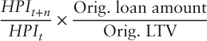 |
 |
= Loan origination period | |
 |
= Current period |
The case study highlights the analysis of involuntary prepayment rates (borrower default) based on the following predictor variables:
- Loan age
- Original loan-to-value ratio
- Home prices—measured via the borrower's updated loan-to-value ratio
- Borrower's credit score
- SATO
20.1.1 Influence of Loan-to-Value Ratio on the Expected Default Rate
Default modeling begins with an analysis of borrower's original and updated loan-to-value ratio (recall from Chapter 8.5 the three data types: categorical, continuous, and time dependent):
- The borrower's original loan-to-value ratio is a continuous variable.
- The borrower's updated loan-to-value ratio is a time-dependent variable.
Departing somewhat from the modeling techniques presented in Chapter 8, the functional form of the original and updated loan-to-value ratios are explored by transforming both from continuous to categorical variables by “binning” the data into discrete values. To summarize, the modeling techniques presented in this chapter differ from those presented in Chapter 8 in the following manner:
- A fully parametric model is used (logistic regression) rather than the semi-parametric Cox proportional hazard model.
- The functional form of the continuous variables are explored by transforming those variables to categorical variables rather than via residual analysis.
Figure 20.3 presents default frequency by original loan to value. Notice default rates tend to go up as the original loan-to-value ratio increases, suggesting the following:
- A borrower that is able to make a substantial down payment represents a superior credit risk relative to one unable to make a significant down payment.
- A borrower with little to no equity is more likely to default than one with a significant equity share, particularly in a declining home price environment.
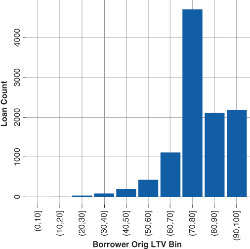
Figure 20.3 Default Freq. Orig. LTV
Figure 20.4 is a histogram of borrower default given the updated loan-to-value ratio. The distribution is skewed right indicating that a borrower in a negative equity position is more likely to default than one in a positive equity position. The fact that the borrower default declines as homeowner's equity increases suggests the following:
- Rising home prices and the wealth effect associated with home equity gains act to reduce default rates
- A borrower facing default is more likely to sell to realize a gain than a loss. Consequently, the default becomes a voluntary repayment.
- Positive home equity suggests a borrower with greater financial flexibility, thereby reducing the probability of default.
- Declining home prices may trigger a strategic default on the part of the borrower. That is, a borrower transitioning from a positive to negative equity position due to declining home prices may decide to simply default and walk away from his obligation.
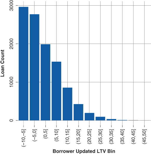
Figure 20.4 Default Freq. Updated LTV
Figures 20.3 and 20.4 provide a visual representation of default. Unfortunately, one is unable to determine relative risk—a comparison of risk between the levels of updated and original loan-to-value ratios. Table 20.1 summarizes the results of a logistic regression of original and updated loan-to-value ratio. Loan age is a predictor in the model and as before a spline is used to model its functional form. The borrower's updated loan to value is measured by the change from the original to the current loan-to-value ratio.
- Both the intercept and the loan age are significant at the 99.0% confidence level.
- An original loan-to-value ratio below 80% is not a significant predictor of borrower default at the 99% confidence level. The astute observer will notice an original loan-to-value ratio greater than 100% is not significant due to the low loan count within the category.
- The borrower's updated loan-to-value ratio is a significant predictor of default at the 99.0% confidence level across all categories.
Table 20.1 Logistic Default Model
| Estimate | Std. Error | Z value | Pr( Z Z ) ) |
|
| (Intercept) | −5.0277 | 0.5861 | −8.58 | 0.0000 |
| ns(LoanAge, df = 3)1 | 1.8378 | 0.0558 | 32.94 | 0.0000 |
| ns(LoanAge, df = 3)2 | 2.1245 | 0.1227 | 17.32 | 0.0000 |
| ns(LoanAge, df = 3)3 | −0.4304 | 0.0987 | −4.36 | 0.0000 |
| OrigLTVBin(10,20] | −1.1203 | 0.6571 | −1.70 | 0.0882 |
| OrigLTVBin(20,30] | −1.1060 | 0.6069 | −1.82 | 0.0684 |
| OrigLTVBin(30,40] | −0.7438 | 0.5921 | −1.26 | 0.2091 |
| OrigLTVBin(40,50] | −0.5201 | 0.5877 | −0.88 | 0.3762 |
| OrigLTVBin(50,60] | −0.1379 | 0.5854 | −0.24 | 0.8137 |
| OrigLTVBin(60,70] | 0.4592 | 0.5842 | 0.79 | 0.4318 |
| OrigLTVBin(70,80] | 0.7016 | 0.5836 | 1.20 | 0.2293 |
| OrigLTVBin(80,90] | 1.5922 | 0.5839 | 2.73 | 0.0064 |
| OrigLTVBin(90,100] | 1.8274 | 0.5839 | 3.13 | 0.0017 |
| OrigLTVBin(100,110] | −5.4311 | 40.2717 | −0.13 | 0.8927 |
| ChgLTV(−5,0] | −0.4350 | 0.0276 | −15.75 | 0.0000 |
| ChgLTV(0,5] | −1.1050 | 0.0313 | −35.29 | 0.0000 |
| ChgLTV(5,10] | −0.8213 | 0.0333 | −24.67 | 0.0000 |
| ChgLTV(10,15] | −0.8203 | 0.0405 | −20.28 | 0.0000 |
| ChgLTV(15,20] | −0.9736 | 0.0534 | −18.23 | 0.0000 |
| ChgLTV(20,25] | −1.1243 | 0.0747 | −15.04 | 0.0000 |
| ChgLTV(25,30] | −1.3568 | 0.1025 | −13.24 | 0.0000 |
| ChgLTV(30,35] | −1.8167 | 0.1591 | −11.42 | 0.0000 |
| ChgLTV(35,40] | −2.2390 | 0.2702 | −8.29 | 0.0000 |
| ChgLTV(40,45] | −2.5544 | 0.4510 | −5.66 | 0.0000 |
| ChgLTV(45,50] | −1.5626 | 0.5115 | −3.05 | 0.0023 |
The model indicates original loan-to-value ratios greater than or equal to 80% are significant predictors of default, while lower loan-to-value ratios are not significant predictors of default.
Figures 20.5 and 20.6 are an examination of the odds ratios and their standard errors, which are obtained by exponentiation of each. The confidence interval of many of the odd ratios overlap, suggesting they may not be significantly different. For example, at the 95% confidence level  , the OrigLTVBin(80,90] and OrigLTVBin(90, 100] odds ratios overlap; thus, these ratios (coefficients) may not be significantly different.
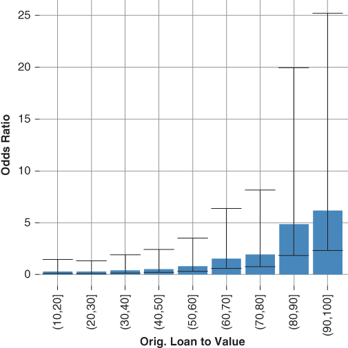
Figure 20.5 Orig. LTV Odds Ratio

Figure 20.6 Updated LTV Odds Ratio
The change in borrower equity is also a significant predictor of the default. Despite the lower standard errors of the coefficients, they still overlap, suggesting the bins used are not significantly different. For example, the (10,15], (15,20], (20,25] odds ratios overlap, indicating a potential lack of statistical difference between the coefficients.
Both the original loan-to-value ratio and the updated loan-to-value ratio, after adjusting for loan seasoning (loan age), are significant predictors of default. Nonetheless, the analysis of the significance of these predictors and their standard errors suggests combining and reducing the number of transformations of both original and updated loan-to-value ratios into fewer categorical variables. Specifically:
- The original loan-to-value ratio is binned using cut-points of 0%, 80%, 90%, and 110%, creating the following three levels within the original loan-to-value categorical variable (0,80], (80,90], and (90,110].
- The change in loan to value is binned, creating the following levels within the updated loan-to-value categorical variable (−10,5], (−5,0], (0,15], (15,30], and (30,50].
The idea is simple; the analysis presented in Table 20.1 suggests some bins are not significantly different in terms of their influence on borrower default rates, nor is the number of observations (loan count) within the bin sufficient to determine a reliable coefficient. The strategy of combining bins achieves the following:
- The number of levels within each categorical variable is reduced.
- The statistical significance of each bin (level) increases.
- Each bin (level) is significantly different relative to the others.
Once a proper transformation of a continuous variable to a categorical variable is complete, the model is refit and the investor may extract the functional form of those variables under investigation. The functional form is determined by examining and plotting the odds ratio of the levels within each explanatory variable.
Table 20.2 presents the results of the model after combining levels within each categorical variable. The predictive variables of the model are significant beyond the 99% confidence level, with the exception of the ChgLTV(20,35] categorical variable—which is significant beyond the 90% confidence interval. Notice, the levels of each categorical variable have been ordered such that the referent or baseline defines a borrower with an original loan to value between 80% and 90% and a change in the borrower's loan-to-value ratio between 0% and 15% (recall section 8.5.1). Once the model is fit, the functional form of both original loan to value and updated loan-to-value ratios may be explored by plotting the odds ratio of each level with the predictive variable.
Table 20.2 Logistic Default Model
| Estimate | Std. Error | z value | Pr( z z ) ) |
|
| (Intercept) | −4.4335 | 0.0532 | −83.26 | 0.0000 |
| ns(LoanAge, df = 3)1 | 1.8286 | 0.0558 | 32.76 | 0.0000 |
| ns(LoanAge, df = 3)2 | 2.2912 | 0.1200 | 19.09 | 0.0000 |
| ns(LoanAge, df = 3)3 | −0.3292 | 0.0970 | −3.39 | 0.0007 |
| OrigLTVBin(0,80] | −1.1517 | 0.0260 | −44.21 | 0.0000 |
| OrigLTVBin(90,110] | 0.2342 | 0.0320 | 7.32 | 0.0000 |
ChgLTV( 5] 5] |
0.9377 | 0.0259 | 36.18 | 0.0000 |
| ChgLTV(−5,0] | 0.4535 | 0.0254 | 17.85 | 0.0000 |
| ChgLTV(15,30] | −0.0847 | 0.0413 | −2.05 | 0.0406 |
20.1.2 Original Loan-to-Value Odds Ratio
Figure 20.7 plots the original loan-to-value odds ratios and their respective confidence intervals. The confidence intervals around the odds ratios do not overlap, indicating they are significantly different.
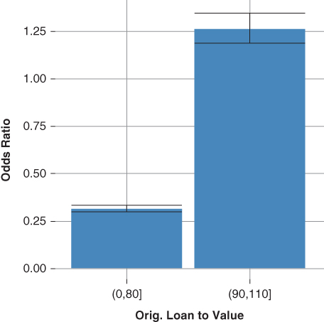
Figure 20.7 Orig. Loan-to-Value Odds Ratio
The interpretation of the odds ratio is straightforward, relative to the referent borrower (original loan to value between 80% and 90%).
- A borrower with a loan-to-value ratio less than 80% is 0.30 times as likely to default.
- A borrower with a loan-to-value ratio greater than 90% is 1.26 times as likely to default.
20.1.3 Updated Loan-to-Value Odds Ratio
Figure 20.8 plots the combined updated loan-to-value odds ratios and their respective confidence intervals. The updated loan-to-value ratio is an example of an external time dependent variable, described in section 8.5.3. The figure indicates that the updated loan-to-value ratio is a decreasing exponential function. That is, the likelihood of default decreases exponentially as the borrower's updated loan-to-value ratio declines. The interpretation of the odds ratios is as follows:
- A borrower with a loan-to-value ratio between 80% and 90% who experiences a negative change between −10% and −5% is 2.5 times more likely to default than a borrower who experiences a positive change in equity between 0% and 15%.
- A borrower with a loan-to-value ratio between 80% and 90% who experiences a negative change between −5% and 0% is 1.5 times more likely to default than a borrower who experiences a positive change in equity between 0% and 15%.
- A borrower with a loan-to-value ratio between 80% and 90% who experiences a positive equity change between 15% and 30% is .90 times less likely to default than a borrower who experiences a positive equity change between between 0% and 15%.
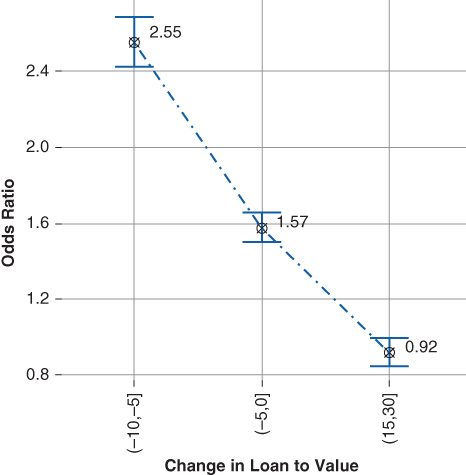
Figure 20.8 Change in Loan-to-Value Odds Ratio
Clearly the risk of default increases as the borrower's equity position deteriorates. At first blush, one may be tempted to attribute the increased risk of default to strategic defaults—the case when a borrower in a negative equity position simply walks away from the home. The strategic default conclusion is too simplistic. Typically, a decline in home prices is symptomatic of a broader economic decline. Consequently, the default may have been triggered by an event such as a job loss, which—although it could be related to the decline in the borrower's equity position—is not a strategic default.
20.2 Other Variables Influencing Borrower Default
The investor may choose to add additional variables to the default model, such as:
-
The quality of the issuer's loan underwriting process. Generally, the quality of the issuer's loan underwriting process, either easy or conservative, will manifest itself as a higher or lower baseline default curve. The investor may choose to adopt an individual default model for each issuer, or alternatively, she may choose to subjectively score each issuer's underwriting process, thereby including her judgment in the model.
The loan origination channel includes the following:
- Retail: The issuer may originate loans through its own trained employees.
- Correspondent: A correspondent agrees to underwrite loans in accordance with the issuer's underwriting matrix and practices (acts as the issuer's agent). In return, the issuer agrees to purchase loan packages from the correspondent.
-
Broker: A broker may submit a loan package to a number of lenders.
Simply from a standpoint of quality control, one would expect the retail channel to exhibit the highest level of credit quality, followed by the correspondent channel, then the broker channel. Consequently, one would think the retail channel may exhibit the lowest frequency of default, while the correspondent and broker channels may exhibit higher ones.
- Measures of borrower financial flexibility, these include:
- The borrower's credit score, which may be assigned by the loan underwriter according to an internal credit model or simply a credit score reported by any of the credit monitoring/reporting services. A borrower with a high credit score exhibits a willingness to pay—the first key underwriting standard—and as a result, one would expect those borrowers with higher credit scores to exhibit a lower incidence of default.
- A borrower with a lower debt-to-income ratio has greater financial flexibility than one with a higher debt-to-income ratio and exhibits a greater ability to pay—the second key underwriting standard. Consequently, one would expect a borrower with a lower debt to income ratio to exhibit a lower incidence of default.
- Property occupancy—either owner or investor. One would expect investor owned properties to exhibit a higher incidence of default than those that are owner occupied as the former may be subject to a greater risk of strategic default.
20.2.1 Borrower Credit Score
Including the borrower's credit score in the default model follows the method previously outlined. The borrower's credit score is binned and the model is refit. The coefficients are translated to odds ratios. Both the odds ratios and standard errors are plotted and examined. Figure 20.9 plots the odds ratios of borrower original credit score and their associated confidence intervals:
- The baseline borrower credit score is (750,800]. Thus, the model's baseline borrower possess the following characteristics:
- The original loan to value is between 80% and 90%.
- The change in loan to value is between 0% and 15%.
- The original credit score is between 750 and 800.
- The confidence intervals around each coefficient do not overlap each other, indicating the coefficients are significantly different.
- Credit score is decreasing exponential function. For example, all else equal:
- A borrower with an original credit score between 300 and 550 is 37 times more likely to default than the baseline borrower, suggesting the borrower is almost certain to default.
- A modest downward drift in borrower credit score increases the likelihood of default. For example, underwriting a borrower with an original credit score between 700 and 750 increases likelihood of default by 2.8 times.
- A borrower with an original credit score between 800 and 850 is less than half as likely to default as the baseline borrower.
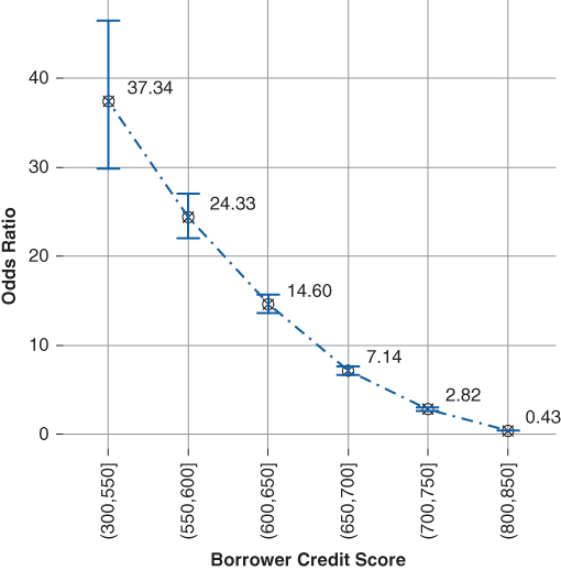
Figure 20.9 Borrower Credit Score Odds Ratio
20.2.2 Borrower Debt to Income
The borrower's debt to income ratio at origination is binned and the model is fit again. Figure 20.10 plots the borrower's debt to income odds ratio and their associated confidence intervals. Addition of the borrower's debt to income ratio improves the overall model fit by a modest amount. However, most likely the borrower's debt to income ratio will be somewhat correlated to his credit score, as a lower ratio indicates a lower level of debt service and by extension implies a borrower with a stronger credit profile.
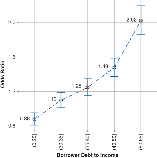
Figure 20.10 Borrower Debt to Income Odds Ratio
The borrower's debt to income ratio appears linear with a kink at the (40,50] cut point. Beyond the (40,50] cut point the slope increases, suggesting a higher relative frequency of default beyond a 40 debt to income ratio. The increase in the slope of the function beyond a 40 debt to income ratio is likely due to the lower overall financial flexibility of the borrower.
20.3 Spread at Origination (SATO) and Default
Recall, from Chapter 11, spread at origination (SATO) captures the spread or premium paid by the borrower above the current “prime” lending rate at the time of origination. A high SATO implies a borrower with a weaker credit profile, which results in lower relative turnover rates and less responsiveness to economic incentives to refinance. Given a higher SATO is associated with lower voluntary repayments it stands to reason that SATO may also act as a predictor on the frequency of default.
SATO is a significant predictor of default and the initial investigation of the model suggests a SATO-based model is preferable over a model including borrower credit score and debt to income because measuring the premium paid by the borrower over the “prime” mortgage lending rate at the time of origination captures the combination of factors that determine his credit profile. SATO is an exponentially increasing function on a borrower's expected default rate:
- A borrower required to pay an additional 25 to 75 basis points above the prime lending rate is 1.4 times more likely to default than one who is able to finance at the prime lending rate.
- The expected default rate increases exponentially as SATO increases. A borrower required to pay 125 to 175 basis points over the prime lending rate is 2.5 times more likely to default than one who is able to finance at the prime lending rate.

Figure 20.11 Borrower SATO Odds Ratio
20.4 Default Model Selection
Figure 20.12 compares the credit score (720) and debt to income ratio (25) model versus the SATO model (75 basis points). The average SATO of the borrower cohort with a 720 credit score and 25 debt to income ratio is 75 basis points, suggesting each model should return similar predictions—as is the case.
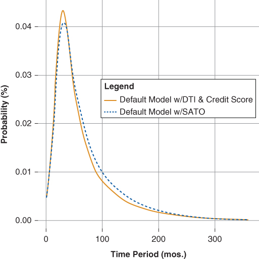
Figure 20.12 Default Model Comparison
A confusion matrix, Table 20.3, is calculated and used to decide which model to deploy.
- The accuracies of the models are comparable, suggesting that either model may be useful to predict the incidence of default.
- The sensitivities of both models are comparable. Sensitivity, in this case, measures the model's ability to correctly identify the incidence of default.
- The specificity of the DTI and credit score model is higher than that of the SATO model. Specificity relates to a model's ability to exclude the incidence of default correctly.
Table 20.3 Confusion Matrix Model Comparison
| Model w/ DTI | Model w/ SATO | |||||||||||||||||||
|
|
|||||||||||||||||||
| Accuracy | 0.953 | 0.958 | ||||||||||||||||||
| 95% CI | (0.958, 0.960) | (0.957, 0.959) | ||||||||||||||||||
| No Information Rate | 0.957 | 0.958 | ||||||||||||||||||
| Sensitivity | 0.997 | 0.999 | ||||||||||||||||||
| Specificity | 0.101 | 0.050 | ||||||||||||||||||
| Pos. Pred. Value | 0.961 | 0.959 | ||||||||||||||||||
| Neg. Pred. Value | 0.661 | 0.693 | ||||||||||||||||||
| Prevalence | 0.957 | 0.957 | ||||||||||||||||||
| Detection Rate | 0.954 | 0.956 | ||||||||||||||||||
| Detection Prevalence | 0.993 | 0.996 | ||||||||||||||||||
| Balance Accuracy | 0.549 | 0.524 |
The analysis suggests the SATO model overstates the incidence of default and results in a higher number of false positives (defaults when there is no default). That is, the SATO model has a higher level of sensitivity and lower level of specificity. However, both models seem comparable in performance and the analysis suggests SATO can be used effectively to predict the frequency of default. The advantages of the SATO model are:
- It requires fewer inputs than the DTI and credit score model. Thus, from a data management standpoint the model is easier to maintain.
- It does not rely on the issuer's loan level disclosure. Often loan level disclosure data may be incomplete or inaccurate due to human error or fraud whereas the SATO model relies on market inputs, the “prime” mortgage lending rate at the time of origination and the borrower's note rate.
Figure 20.13 illustrates the model's projection given the baseline SATO (75 basis points) and a high SATO (300 basis points) notice the influence of a higher SATO on the incidence of default.
- The higher SATO odds ratios begin at 0.01 in the first month compared to the lower SATO odds ratios whose odds begin at 0.0 in the first month.
- By month 30, the higher SATO odds ratio reaches a peak of 0.10 compared to that of the lower SATO odds ratio that reaches a peak of 0.04.
- Throughout most of the life of the loan, the higher SATO exhibits a higher expected default rate, indicating the borrower's weaker overall credit and lack of financial flexibility relative to the lower SATO borrower.
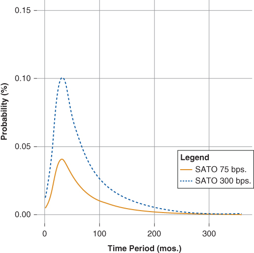
Figure 20.13 Default Model SATO Comparison
The analysis presented indicates a default model based on the following variables:
- Loan seasoning. The expected default rate starts relatively low and increases as the loan seasons reaching a peak around month 30. Thereafter, the expected default rate begins to decline.
- Borrower's initial equity or down payment. A higher down payment suggests a financially stronger borrower than one with a lower down payment.
- Change in the borrower's equity. A borrower migrating from a positive equity position to a negative equity position is 1.5 to 2.5 times more likely to default than a borrower remaining in a positive equity position.
- SATO or spread to the prime lending rate at the time of origination. A higher SATO suggests a borrower with a weaker credit profile and by extension a higher expected default rate.
This chapter presented the analysis of mortgage default using logistic regression as an a alternative to the Cox proportional hazard model presented in Chapter 8. The modeling differences are:
- The functional form of the predictor variables are explored by plotting the odds ratio rather than through residual analysis presented in Chapter 8.
- The logistic regression model is parametric and can be used to predict beyond the last observed point.