If we want to be nice to our machine learning algorithm, we will provide it with features that are not dependent on each other, yet highly dependent on the value to be predicted. It means that each feature adds some salient information. Removing any of the features will lead to a drop in performance.
If we have only a handful of features, we could draw a matrix of scatter plots – one scatter plot for every feature-pair combination. Relationships between the features could then be easily spotted. For every feature pair showing an obvious dependence, we would then think whether we should remove one of them or better design a newer, cleaner feature out of both.
Most of the time, however, we have more than a handful of features to choose from. Just think of the classification task where we had a bag-of-words to classify the quality of an answer, which would require a 1,000 by 1,000 scatter plot. In this case, we need a more automated way to detect the overlapping features and a way to resolve them. We will present two general ways to do so in the following subsections, namely filters and wrappers.
Filters try to clean up the feature forest independent of any machine learning method used later. They rely on statistical methods to find out which of the features are redundant (in which case, we need to keep only one per redundant feature group) or irrelevant. In general, the filter works as depicted in the workflow shown in the following diagram:

Using correlation, we can easily see linear relationships between pairs of features, which are relationships that can be modeled using a straight line. In the graphs shown in the following screenshot, we can see different degrees of correlation together with a potential linear dependency plotted as a red dashed line (a fitted one-dimensional polynomial). The correlation coefficient  at the top of the individual graphs is calculated using the common Pearson correlation coefficient (the Pearson
  value) by means of the
 pearsonr() function of scipy.stat.
Given two equal-sized data series, it returns a tuple of the correlation coefficient values and the p-value, which is the probability that these data series are being generated by an uncorrelated system. In other words, the higher the p-value, the less we should trust the correlation coefficient:
>> from import scipy.stats import pearsonr
>> pearsonr([1,2,3], [1,2,3.1])
>> (0.99962228516121843, 0.017498096813278487)
>> pearsonr([1,2,3], [1,20,6])
>> (0.25383654128340477, 0.83661493668227405)
In the first case, we have a clear indication that both series are correlated. In the second one, we still clearly have a non-zero  value.
However, the p-value basically tells us that whatever the correlation coefficient is, we should not pay attention to it. The following output in the screenshot illustrates the same:
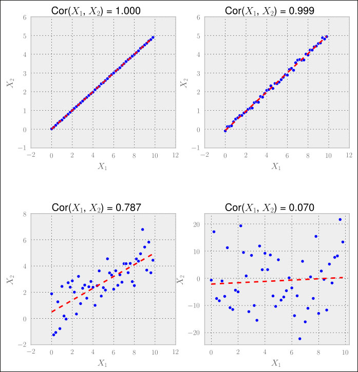
In the first three cases that have high correlation coefficients, we would probably want to throw out either  or
or  since they seem to convey similar if not the same information.
In the last case, however, we should keep both features. In our application, this decision would of course be driven by that p-value.
Although it worked nicely in the previous example, reality is seldom nice to us. One big disadvantage of correlation-based feature selection is that it only detects linear relationships (a relationship that can be modeled by a straight line). If we use correlation on non-linear data, we see the problem. In the following example, we have a quadratic relationship:
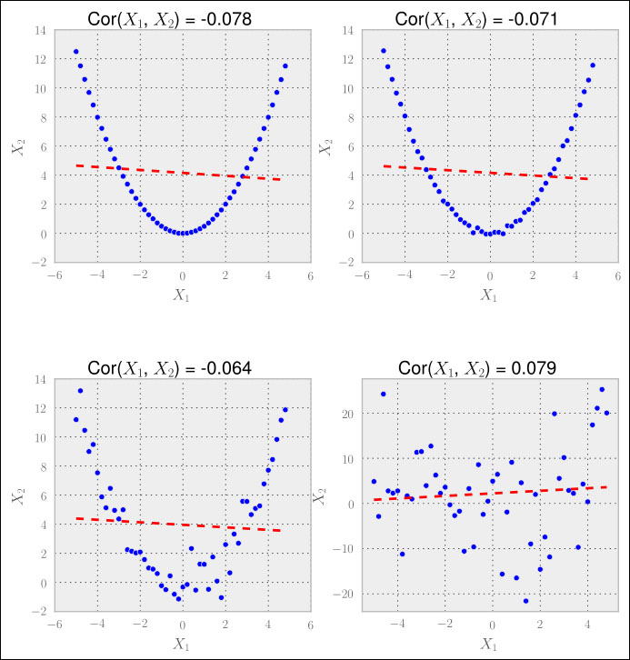
Although the human eye immediately sees the relationship between X1 and X2 in all but the bottom-right graph, the correlation coefficient does not. It is obvious that correlation is useful to detect linear relationships, but fails for everything else.
For non-linear relationships, mutual information comes to the rescue.
When looking at the feature selection, we should not focus on the type of relationship as we did in the previous section (linear relationships). Instead, we should think in terms of how much information one feature provides, given that we already have another.
To understand that, let us pretend we want to use features from the feature set house_size, number_of_levels, and avg_rent_price to train a classifier that outputs whether the house has an elevator or not. In this example, we intuitively see that knowing house_size means we don't need number_of_levels anymore, since it somehow contains redundant information. With avg_rent_price, it is different as we cannot infer the value of rental space simply from the size of the house or the number of levels it has. Thus we would be wise to keep only one of them in addition to the average price of rental space.
Mutual information formalizes the previous reasoning by calculating how much information two features have in common. But unlike correlation, it does not rely on a sequence of data, but on the distribution. To understand how it works, we have to dive a bit into information entropy.
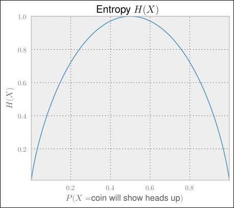
Let's assume we have a fair coin. Before we flip it, we will have maximum uncertainty as to whether it will show heads or tails, as both have an equal probability of 50 percent. This uncertainty can be measured by means of Claude Shannon's information entropy:

In our fair coin scenario, we have two cases: let  be the case of heads and
  the case of tails, with
  .
.
Thus, we get the following:

Now imagine we knew upfront that the coin is actually not that fair, with the heads side having a 60 percent chance of showing up after flipping:

We can see that this situation is less uncertain. The uncertainty will decrease the farther we get from 0.5, reaching the extreme value of 0 for either a 0 percent or 100 percent chance of the head showing up, as we can see in the following graph:
We will now modify the entropy  by applying it to two features instead of one, such that it measures how much uncertainty is removed from X when we learn about Y. Then we can catch how one feature reduces the uncertainty of another.
For example, without having any further information about the weather, we are totally uncertain whether it is raining outside or not. If we now learn that the grass outside is wet, the uncertainty has been reduced (we will still have to check whether the sprinkler had been turned on).
More formally, mutual information is defined as:

This looks a bit intimidating, but is really not more than sums and products. For instance, the calculation of  is done by binning the feature values and then calculating the fraction of values in each bin. In the following plots, we have set the number of bins to 10.
In order to restrict mutual information to the interval [0,1], we have to divide it by their added individual entropy, which gives us the normalized mutual information:

The nice thing about mutual information is that unlike correlation, it is not looking only at linear relationships, as we can see in the following graphs:
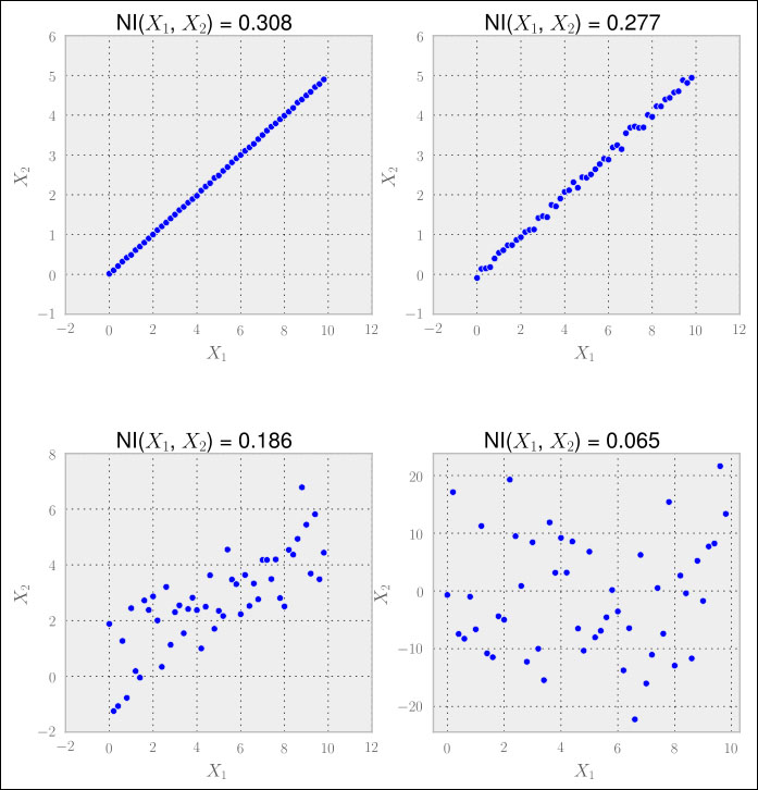
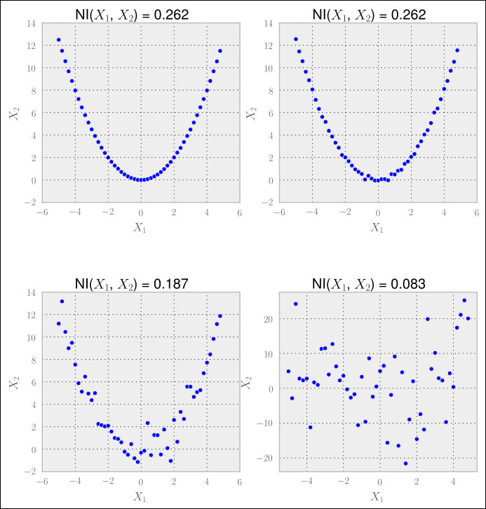
Hence, we have to calculate the normalized mutual information for all feature pairs. For every pair having a very high value (we would have to determine what that means), we would then drop one of them. In case we are doing regression, we could drop the feature that has a very low mutual information with the desired result value.
This might work for a small set of features. At some point, however, this procedure can be really expensive, as the amount of calculation grows quadratically since we are computing the mutual information between feature pairs.
Another huge disadvantage of filters is that they drop features that are not useful in isolation. More often than not, there are a handful of features that seem to be totally independent of the target variable, yet when combined together, they rock. To keep these, we need wrappers.
While filters can tremendously help in getting rid of useless features, they can go only so far. After all the filtering, there might still be some features that are independent among themselves and show some degree of dependence with the result variable, but yet they are totally useless from the model's point of view. Just think of the following data, which describes the XOR function. Individually, neither A nor B would show any signs of dependence on Y, whereas together they clearly do:
|
A |
B |
Y |
|---|---|---|
|
0 |
0 |
0 |
|
0 |
1 |
1 |
|
1 |
0 |
1 |
|
1 |
1 |
0 |
So why not ask the model itself to give its vote on the individual features? This is what wrappers do, as we can see in the following process chart diagram:
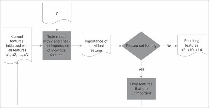
Here we have pushed the calculation of feature importance to the model training process. Unfortunately (but understandably), feature importance is not determined as a binary but as a ranking value. So we still have to specify where to make the cut – what part of the features are we willing to take and what part do we want to drop?
Coming back to Scikit-learn, we find various excellent wrapper classes in the sklearn.feature_selection package. A real workhorse in this field is RFE, which stands for recursive feature elimination. It takes an estimator and the desired number of features to keep as parameters and then trains the estimator with various feature sets as long as it has found a subset of the features that are small enough. The RFE instance itself pretends to be like an estimator, thereby, wrapping the provided estimator.
In the following example, we create an artificial classification problem of 100 samples using the convenient make_classification() function of datasets. It lets us specify the creation of 10 features, out of which only three are really valuable to solve the classification problem:
>>> from sklearn.feature_selection import RFE
>>> from sklearn.linear_model import LogisticRegression
>>> from sklearn.datasets import make_classification
>>> X,y = make_classification(n_samples=100, n_features=10, n_informative=3, random_state=0)
>>> clf = LogisticRegression()
>>> clf.fit(X, y)
>>> selector = RFE(clf, n_features_to_select=3)
>>> selector = selector.fit(X, y)
>>> print(selector.support_)
[False  True False  True False False False False  True False]
>>> print(selector.ranking_)
[4 1 3 1 8 5 7 6 1 2]
The problem in real-world scenarios is, of course, how can we know the right value for n_features_to_select? Truth is, we can't. But most of the time, we can use a sample of the data and play with it using different settings to quickly get a feeling for the right ballpark.
The good thing is that we don't have to be that exact when using wrappers. Let's try different values for n_features_to_select to see how support_ and ranking_ change:
|
n_features_to_select |
support_ |
ranking_ |
|---|---|---|
|
1 |
[False False False True False False False False False False] |
[ 6 3 5 1 10 7 9 8 2 4] |
|
2 |
[False False False True False False False False True False] |
[5 2 4 1 9 6 8 7 1 3] |
|
3 |
[False True False True False False False False True False] |
[4 1 3 1 8 5 7 6 1 2] |
|
4 |
[False True False True False False False False True True] |
[3 1 2 1 7 4 6 5 1 1] |
|
5 |
[False True True True False False False False True True] |
[2 1 1 1 6 3 5 4 1 1] |
|
6 |
[ True True True True False False False False True True] |
[1 1 1 1 5 2 4 3 1 1] |
|
7 |
[ True True True True False True False False True True] |
[1 1 1 1 4 1 3 2 1 1] |
|
8 |
[ True True True True False True False True True True] |
[1 1 1 1 3 1 2 1 1 1] |
|
9 |
[ True True True True False True True True True True] |
[1 1 1 1 2 1 1 1 1 1] |
|
10 |
[ True True True True True True True True True True] |
[1 1 1 1 1 1 1 1 1 1] |
We see that the result is very stable. Features that have been used when requesting smaller feature sets keep on getting selected when letting more features in. Finally we rely on our train/test set splitting to warn us when we go in the wrong direction.