
Congratulations, you made it! Whether you are a novice or last year’s Financial Modelling World Champion (someone needs to explain that title to me), hopefully you learned something as we braved the common functions used in financial modelling.
I make no apologies that certain functions were not there, such as FACTDOUBLE, IPMT, IRR, MIRR, NPV, PMT, PPMT, RATE, ROMAN, XIRR and XNPV (and plenty more) were not discussed. Many of them have issues; others are just simpler to derive from first principles; some just couldn’t make the final cut for this book. Having said that, I might leave you with one final tip. If profits are way down on budgets, rather than issue profit warnings, have you considered producing your lacklustre outputs using the ROMAN function?
Jokes aside, maybe we should move on.
Apart from functions, you should also familiarise yourself with various key functionalities of Excel often required for developing financial models. Just as with functions, I am going to discuss some aspects that you may consider you understand fully already. Again, I’d like to encourage you to stick with the programme, as whether you are a novice or an expert, hopefully, there may be some useful tips for all.
In this section, I plan to explain the merits (or otherwise) of each of the following:
| •Absolute referencing | •Data validation |
| •Number formatting | •Data Tables |
| •Styles | •Goal Seek and Solver |
| •Conditional formatting | •Hyperlinks. |
| •Range names |
If nothing else, this should provide useful reference material as we make sure we have the complete toolkit for putting together a “Best Practice” financial model.
As my editor said to me recently, “are you absolutely sure you need this section?” (I said no such thing - Editor.) Some people say that financial modelling may be all about the dollar signs - well, they may be possibly right in more ways than one.
Consider the following situation:

In this example, I have created data in cells C4:H9 inclusive and then written a formula in cell C14 linking to cell C4 (a bit of an incendiary reference, I know). If I were to copy this formula down and across over a similarly dimensioned range, I would get the following result:

As the formula is copied down and / or across, so the reference moves in a corresponding fashion. This is known as relative referencing and forms the cornerstone of formula construction whenever a modeller refers to another location in the same workbook.
This is not what happens when you refer to another workbook:

becomes

once copied down and across as before. The default for external references is this absolute referencing.
It is the dollar ($) signs that do the damage. These can be added or removed by directly typing them into the cell reference or else clicking in the formula bar (alternatively, use the F2 function key) to enable Edit mode and highlight the relevant references and press the F4 function key repeatedly

The dollar sign makes the reference to the right of the sign constant, viz.

It is important that all would-be modellers master this referencing. It is an essential skill as you need to be able to copy formulae down and across ranges with little effort. If you are unsure, try the following exercise. Create the following spreadsheet:

In this example (assuming you have set up the spreadsheet identically to the one illustrated), the aim is to create a “times table” in cells E7:I11 inclusive. The numbers should be equal to
Column Header Number x Row Header Number x Multiplier
So that the formula in the first cell is =D7*E6*C3. All you need to do is add dollar signs to these cell references so that the formula may be copied across and down the range correctly. Have a go now without peeking.
Have you had a go? Here’s my solution below:

The formula I constructed was:
=$D7*E$6*$C$3
i.e. the first reference has the column anchored (so that it always references the correct Row Header), the second reference has the row anchored (so that it always references the appropriate Column Header) and the final reference is fully anchored (that is, it is an absolute reference).
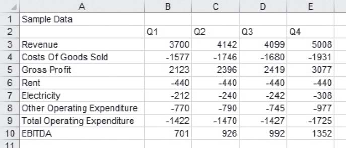
Let’s get a little more sophisticated and deal with more of a real world problem. Imagine you had the following sample business data:

You might wish to create an output which summarises the revenue by business unit. You will need to construct formulae such as
=‘Business Data’!G10
=‘Business Data’!G25
=‘Business Data’!G40, … etc.
If you had, say, 500 of these business units you would have a busy but boring morning ahead of you. Surely there is a simpler way that does not require the implementation of macros?
Actually, I can think of two ways of dealing with this common query and I present both solutions next.
This approach requires the first two formulae to be entered into the output sheet as usual, viz.

In our example, cell B2 contains the formula =‘Business Data’!G10 and cell B3 contains the formula =‘Business Data’!G25 (displayed). Next, edit both formula by typing an apostrophe (‘) before the equals sign in each formula:

Now, these formulae are treated as text and are displayed in the two cells. If you then highlight cells B2:B3 together and copy the formulae down, Excel’s AutoFill feature will copy the cells similar to below:

Now, all we need to do is remove the apostrophes. The first idea that comes to mind is to use ‘Replace…’ (CTRL + H) and replace ‘= with =. Unfortunately, this does not work in all versions of Excel as ‘Replace…’ does not seem to recognise apostrophes in certain instances.
There is a very simple trick to circumvent this problem. With this data still selected, click on the ‘Text to Columns’ button in the ‘Data Tools’ group of the ‘Data’ tab on the Ribbon (ALT + D + E for all versions of Excel or ALT + A + E in Excel 2007 onwards):

This launches the ‘Text to Columns Wizard’ dialog box. In the first step, ensure that the ‘…file type that best describes your data…’ is set to ‘Delimited’:

Then, simply depress the ‘Finish’ button. The spreadsheet will then reinstate the formulae, viz.

Simple!
Now this approach is fairly simple, but has two major drawbacks:
1.This method only works with rows. Using R1C1 formula notation it is possible to create a similar approach for columns, but this technique can be confusing.
2.Once the formulae have been reinstated it is not simple to extend the formulae if necessary. This can be cumbersome where the output summaries may differ period to period for example.
The OFFSET approach counters these issues.
For all those similar to me with the memories of a goldfish (I had to look that up, because I keep forgetting it), the syntax for OFFSET is as follows:
OFFSET(Reference,Rows,Columns,[Height],[Width]).
The arguments in square brackets (Height and Width) can be omitted from the formula. In its most basic form, you will recall OFFSET(Reference,x,y) will select a reference x rows down (-x would be x rows up) and y rows to the right (-y would be y rows to the left) of the reference Reference.
Applying this idea to our example:

Note that the Business Unit data is 15 rows apart (e.g. the first block begins in row 8 and ends in row 22, taking the blank rows into account).
Therefore, I can therefore create one formula I may copy down:

In this example, we have started the formula in cell B2 and copied it down to cell B6. The formula in cell B2 is:
=OFFSET(‘Business Data’!$G$10,ROWS(‘Business Data’!$C$8:$C$22)*(ROWS($A$2:$A2)-1),)
The first reference is the Revenue for Business Unit 1. The Rows reference takes the depth of each block (defined here by ROWS(‘Business Data’!$C$8:$C$22)) multiplied by ROWS($A$2:$A2)-1, e.g. in row 2 this factor will be zero, in row 3 it will be 1, in row 4 it will be 2, etc. This ensures that the next Revenue item is referred to in the next row down.
This may seem complex to begin with, but with practice this idea can be adapted for columns to be skipped as well and to allow for other line items (e.g. Gross Profit, Tax) to be selected instead.
Given that one of the primary purposes of financial modelling is to present numerical data, it is important how numerical data is presented. Cells may be individually formatted using CTRL + 1 or ALT + O + E in all versions of Excel:

Formatting only changes the appearance, not the underlying value, of a cell. For example, if cells A1 and B1 had the number ‘1.4’ typed in but were formatted to zero decimal places, then if cell C1 = A1 + B1, you would truly have 1 + 1 = 3 (well, 1.4 + 1.4 = 2.8 anyway).
This should not be confused with ‘Set precision as displayed’ (from the Ribbon, File -> Excel Options -> Advanced -> When calculating this workbook -> Set precision as displayed).
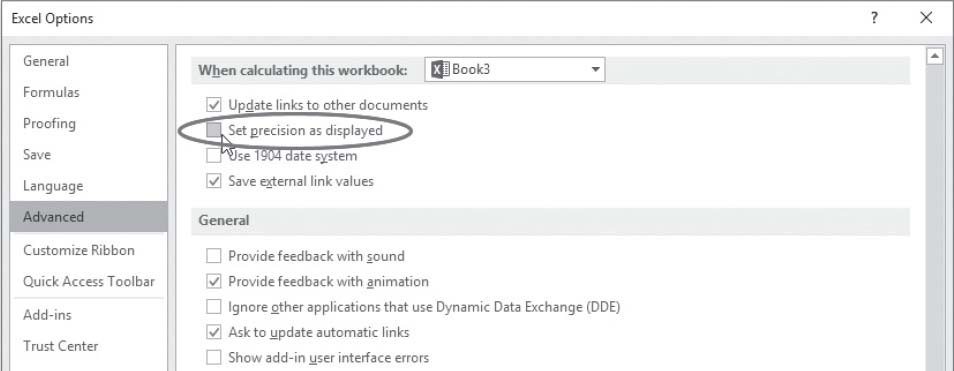
Selecting this option and clicking ‘OK’ will permanently change stored values in cells to whatever format has been selected, including the number of decimal places (e.g. 15.75 formatted to one decimal placed would become precisely 15.8).
From the above diagram, Excel has many built-in number formats that are fairly easy to understand, e.g. Currency, Date, Percentage. The default format is ‘General’ where Excel will endeavour to provide the most appropriate format for the contents. For example, typing ‘3 3/4’ into a cell will result in Excel selecting a mixed format.
But what do you do if you can’t find an appropriate format?
Selecting the ‘Custom’ category activates the ‘Type’ input box and allows between 200 and 250 custom number formats in a particular workbook, depending upon the language version of Excel that has been installed.
The ‘Type’ input box allows up to four aspects of formatting to be specified in a cell. These aspects are referred to as sections and are separated by a semi-colon (;). To ascertain what is contained in each section depends on the total number of sections used, viz.
| No. of Sections | Section Details (assuming no conditions) |
| 1 (min) | All numerical values |
| 2 | Non-negative Numbers; Negative Numbers |
| 3 | Positive Numbers; Negative Numbers; Zero Values |
| 4 (max) | Positive Numbers; Negative Numbers; Zero Values; Text |
To the uninitiated, coding custom number formats may appear incomprehensible. However, understanding the following tables from Microsoft soon puts things into perspective.
| Number Code | Description |
| General | General number format |
| 0 | Digit placeholder (if no number, a ‘0’ will be used to ‘pad’) |
| # | Digit placeholder (does not display extra zeros) |
| ? | Digit placeholder (leaves space for extra zeros, but does not display them) |
| . (decimal point/ full stop) | Decimal point! |
| % | Percentage displayed |
| , (comma) | Thousands separator |
| / | Used to delineate numerator from denominator in Fraction category |
| E+ e+ E- e- | Scientific notation |
| Text Code | Description |
| $ - + / ( ) : space | These characters are displayed in the number. |
| “text” | For other characters, in order to ensure Excel does not misinterpret them, it is best to use enclose the character(s) in quotation marks... |
| \character | ...or precede it with a backslash |
| * | Repeats the next character in the format to fill the column width. Only one asterisk per section of a format is allowed |
| _character | Skips the width of the next character. In particular, this syntax is often used with the closing parenthesis, _) , in a positive number format (when the negative format includes brackets). This allows the values to line up at the decimal point |
| @ | Text placeholder |
| Time Code | Description |
| h | Hours as a number without leading zero (0 to 23) |
| hh | Hours as a number with leading zero (00 to 23) |
| m | Minutes as a number without leading zero (0 to 59) |
| mm | Minutes as a number with leading zero (00 to 59) |
| s | Seconds as a number without leading zero (0 to 59) |
| ss | Seconds as a number with leading zero (00 to 59) |
| [h] | With times only, will increment hours to 24 and beyond |
| [m] | With times only, will increment minutes to 60 and beyond |
| [s] | With times only, will increment seconds to 60 and beyond |
| AM/PM am/pm | Time based on the 12-hour clock [24-hour clock is the default] |
| Miscellaneous Code | Description |
| [Black], [Blue], [Cyan], [Green], [Magenta], [Red], [White], [Yellow] | Displays the characters in the specified colours |
| [Color n] | Displays the characters in a specified colour, where n is a value from 1 to 56, and refers to the nth colour in the color palette |
| ; | Delineates a section |
| [Condition Value] | Condition may be any one of the comparison operators, <, >, =, <=, >=, <> and Value may be any number. A number format may contain up to two conditions |
Allow me to go through several examples.
[Blue]$* _(#,##0.0,_0_);[Red]$* (#,##0.00,);[Color 7]\-_._0_0_);[Cyan]@*.”is text”
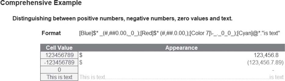
This format has all four sections, so the first section, [Blue]$* _(#,##0.0,_0_), specifies the formatting for positive numbers. In this case, positive numbers will be formatted blue and be preceded with a $ sign. Note the use of the asterisk followed by a space: this means that the cell width will be ‘padded out’ with spaces so that the dollar sign will be pushed to the very left of the cell and the number formatting will be to the very right. _( is not necessary, strictly speaking, but ensures there is space made for an open bracket, even though there is no such character shown. #,##0.0, ensures positive numbers contain thousand separators (where needed) and displays the number to the nearest 0.1 of a thousand. Two commas at the end would have the number displayed to the nearest 0.1 of a million, and so on. Finally, the _0_) requires Excel to maintain enough space at the right end of a cell for a digit (not necessarily zero) and a close bracket. It should be noted that a separate underscore is required for each character that is to be allowed for.
The second section, [Red]$* (#,##0.00,), specifies the formatting for negative numbers. It is similar to the first section, but colours the number red, reports numbers to 0.01 of a thousand and encloses it in brackets.
The third section, [Color 7]\-_._0_0_), specifies the formatting for zero values. This colours zero values “Color 7” which is a delightful pink in Excel’s standard color palette. I am a great believer in using a dash, generated by using \- here, to denote zero as it distinguishes a zero value from something that is approximately zero, which can be useful for error checking. The final four underscored characters, _._0_0_), ensure that the dash will line up with the units value of a positive or negative value.
Finally, the fourth section, [Cyan]@*.”is text”, defines how text is to be formatted. If omitted, text is simply formatted as ‘General’, but here it will be coloured cyan. The @ symbol specifies the relative location of the text within the cell (left-hand side of the cell), the *. will ‘fill’ the cell with period characters and “is text” will add these words to the end of the text, right-aligned (note no ‘&’ concatenation is required since these words appear in the formatting only).

Colouring the font and the background the same may hide a cell’s contents on screen, but it will often reappear when printed out (especially if ‘black and white printing’ is selected). By choosing the above formatting (three semi-colons), numbers and text are simply ‘blanked out’ and will only appear in Excel’s formula bar instead.
[>=1000000]#,##0,,”M”;[>=1000]#,##0,”K”;0

Earlier, I mentioned what the four sections mean most commonly. This third example highlights that this is not always the case. Custom number formats allow up to two conditions to be specified. This is because only four sections are allowed for custom number formatting and two are reserved. The fourth section always specifies text formatting and one other section is required to detail how ‘everything else’ (numerically) will be formatted. It is a bit like conditional formatting (see later), just for numbers.
The conditions are included in square brackets such that if the condition is true, the following formatting will be applied. In this example, there are only three sections, so text will be formatted as ‘General’. The first section, [>=1000000]#,##0,,”M”, will format all numbers greater than or equal to a million to the nearest million and add an “M” to the end of the number. Note that the commas effectively make it look like each divided by 1,000.
The second section will only be considered if the first condition is not true, so the order of the two ‘conditional formats’ needs to be thought through. Here, the second section, [>=1000]#,##0,”K”, will format all numbers greater than or equal to a thousand (but necessarily less than a million) to the nearest thousand and add a “K” to the end of the number.
The third and final section, 0, will format all other numbers (every value less than 1,000) to the nearest integer without thousands separator(s).
Using lots of custom number formats in a single workbook uses considerable memory and can slow down the calculation time of an Excel file unnecessarily. Many of these formats are created accidentally. Each time a custom number format is edited, it will generate an additional listing for Custom Category Types. Any custom formats created inadvertently in this manner (that are not being used in the file) should be deleted; good house-keeping is essential.
Do you know the difference between formats and styles, other than formatting is what you do in Excel and style is what I lack? Take the illustration below. How easy is it to find the key data, or see which cells should be changed to facilitate updated information? Have you ever noticed that spreadsheets built by colleagues do not look similar to your own? How easy are these things in your own spreadsheets? Have I asked enough questions in this paragraph? No?
Later on, I will discuss the four key qualities of a “Best Practice” model, but as a taster, two of these key qualities are consistency and transparency.
•formulae are copied without amendment across rows
•cells with a common purpose (for example, inputs that are assumptions, such as inflation rates) are formatted similarly
•titles are positioned in the same cells in different worksheets
•assumption cells (cells containing data that can be changed by the user to affect model outputs) are unlocked, where all other cells are locked, so that only the assumption cells can be changed.
•assumptions are formatted to be instantly recognisable
•key outputs (for example, totals) can be identified immediately, with their derivation made obvious.

Excel’s ‘Styles’ features can assist with both transparency and consistency. Frequently, the words ‘formats’ and ‘styles’ are used interchangeably, but they are not the same thing. To see this, select any cell in Excel and apply the shortcut keystroke CTRL + 1. As mentioned previously, this shortcut brings up the ‘Format Cells’ dialog box:
Excel has six format properties: Number, Alignment, Font, Border, Fill and Protection. A style is simply a pre-defined set of these various formats. With a little forethought, these styles can be set up and applied to a worksheet cell or range very easily.
Creating your own styles is straightforward with Excel’s Style dialog box. Simply go to the Home tab, click the arrow in the bottom right corner at the very right-hand corner of the ‘Styles’ section:

This expands the section:

You can then select a New Cell Style (see the list at the bottom of the pop-up or ALT + H + J + N), use an existing style or modify an existing style (right-click with the mouse). If you decide to create a new style or edit an existing one, the following dialog box will appear:

Let’s create an assumption format for entering data in dollars. First, select a cell or range of cells. Then, call up the above dialog box by selecting “New Cell Style”. We’ll change the name to ‘Dollar Assumptions” and click the ‘Modify’ or ‘Format’ button (depending upon the version of Excel you have).
The ‘Format Cells’ dialog box reappears:
•Number: select the Currency category, with zero decimal places and apply the ‘$’ symbol
•Alignment: Horizontal - Right (Indent) with zero indent
•Fill: select an ‘easy-on-the-eye’ colour such as pale green
•Protection: uncheck the Locked check box (allows the cell to be changed in a protected worksheet)
•Click ‘OK’ to return to the Style dialog box.
Note that no formats have been ascribed for Font or Border in this example. We don’t want the style to control (that is, overwrite) these properties, so the ‘Style Includes’ check boxes for these two format properties should be unchecked:

This allows you to combine multiple formatting properties in one cell, although there is no point having more than six as you will be overwriting an earlier style otherwise. Returning to the graphic, click on ‘OK’ or ‘Add’. Now that this style has been added, you simply select the range and then click on the style in the Styles gallery on the Home tab.
The main difference between formats and styles becomes obvious when you realise you want to change (update) a style. Call up the Style dialog box in the usual way, modifying the style as required. Click ‘OK’ when finished. Note that every cell in the open workbook that uses this style has automatically updated. Once you start using styles, you will never look back!
You will only want to set up styles once. When you’re finished, simply save the file as a template (.xltx) using File-->Save As (you may wish to delete or remove formatted cells first so that you have a blank workbook). Using File-->New will call up your saved styles.
With very little practice, you will find yourself being able to style worksheets faster than you can say “floccinaucinihilipilification” (I am impressed my spell checker recognises this word!). Returning to our original example, which do you prefer?

Should you have the Styles you want in another workbook, there is a quick way to copy them in. Simply have both workbooks open. Then, in the workbook in which you would like to import the Styles, go to ‘Merge Styles...’ viz.

A dialog box will pop up from which you may select the workbook with the Styles you require.

Click on the correct workbook and then on ‘OK’ and all of the Styles from that workbook will be imported (including any duplicates).
This leads me on to mentioning one issue with Styles. If worksheets or ranges are copied from other workbooks, the Styles from that workbook may be copied across too, leading to hundreds - if not thousands - of Styles you don’t want, artificially bloating the size of your financial model. To delete Styles, you right-click on the Style of your choice and select ‘Delete’ - but this has to be performed one at a time. Yuck!
There are two workarounds to this issue:
•When copying from another workbook, copy the range to be imported (CTRL + C) and then paste special twice. First, in the destination workbook, select where you want the data to go and Paste Special as Formulas (ALT + E + S + F + ENTER) and then Paste Special as Formats (ALT + E + S + T + ENTER).
•Use a macro to delete Styles.
I provide an example of such a macro below. This one allows you to choose which custom (i.e. not those that are built in) Styles should be deleted in the workbook:

This book is not about macros, so forgive me if I only mention them in passing here and there. Essentially, a macro is a coded procedure using the language Visual Basic for Applications (VBA) often used to automate actions. Since Excel 2007, files must not be saved as *.xlsx files (these Excel workbooks will not allow macros). Your best bet is to use a macro-enabled workbook - *.xlsm.
Even then, because macros may execute all sorts of undesirable code, Excel's default setting is set so that macros will not run automatically. To ensure the macro below will work, when you open the file, make sure that you click on "Enable Content" or "Enable Macros" when prompted.
To enter a typed (rather than recorded) macro, open the Visual Basic Editor (ALT + F11), select the file (if more than one open) from the Project Explorer (top left-hand window) and then from the menu, click Insert->Module and type your code into the right-hand pane.

To run the macro, you can go to the View tab and click on the Macros button.
With Excel’s IF function, the contents of a cell can be modified depending upon (a) certain condition(s) being met (i.e. held to be TRUE). However, the formatting or style of the cell cannot be changed in this manner.
Macros are not needed.
First introduced in Excel 97, Conditional Formatting is an Excel feature that indeed allows you to apply formats to a cell or range of cells, and have that formatting change depending on the value of the cell or the value of a corresponding formula. This was one of the features that was given a major overhaul in Excel 2007.
Accessed from the ‘Home’ tab (or ALT + O + D), conditional formatting formats the cell(s) selected depending upon whether a condition is TRUE. In Excel 2003 and earlier versions, conditional formatting would work as follows:

Essentially, as soon as Excel finds a condition that is held, it formats accordingly and stops. If none of the three conditions is met, the underlying format (i.e. the fourth format) is retained.
As explained above, conditional formatting was completely revamped and reinvented in Excel 2007. Located in the ‘Styles’ group of the ‘Home’ tab, the conditional formatting feature has had a raft of new features added:

For instance, inspecting ‘Highlight Cells Rules’ is akin to many of the “Cell Value Is” functionalities of its predecessor, such as Greater Than, Less Than, Between, Equal To, or even More Rules:

Other options are also available: Date Occurring and Duplicate Values. All you have to do is highlight the list, select the option and colour scheme required. No need to concoct hideous formulae such as =IF(COUNTIF($A:$A,$A1)>1,COUNTIF($A$1:$A1,$A1)>1) for locating duplicates, for example.
Users should not be fooled by the easy-to-use Top / Bottom Rules either. Top 10 Items, Top 10%, Bottom 10 Items and Bottom 10% all highlight items that conform to these labels. However, the ‘10’ can be changed to a number of the user’s choice. Who could possibly live without the Bottom 37% Debtors Report, for instance?
Above average and below average data can be highlighted also in one or two clicks and even graded shading of a cell as well. For example, if cells A1:A10 had the values 10, 20, 30, …, 100 respectively, the cells could be filled in as follows:
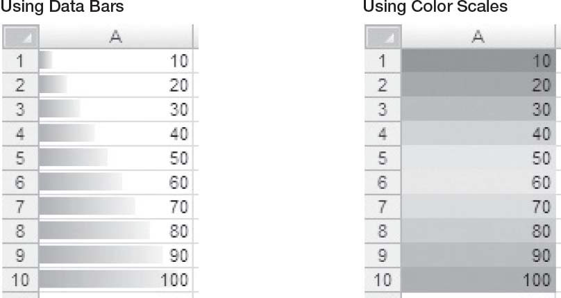
Clearly, looking at the Color Scales example, conditional formatting lends itself neatly to traffic light reporting. This is compounded by Icon Sets that will stratify data into three to five sections using various icons (such as the red, amber and green traffic lights). Given that conditional formatting now permits cells to be sorted dependent upon their background colour (ALT + D + S, then choose ‘Cell Color’ in ‘Sort On’ field), you can make monthly reporting a colourful adventure!
Conditional formatting in Excel 2007 does differ logically from its predecessor.
With Excel 2003 and earlier, as soon as Excel finds a condition that is held it formats accordingly and stops. This can be performed for up three conditions. These days, there is ‘no limit’ and testing does not have to stop (more than one format can be applied in a cell at a time), i.e.

To highlight this, consider the following data set before and after multiple conditional formatting:

No less than four conditional formats have been applied, as can be seen by opening up the Conditional Formatting Rules Manager (ALT + O + D):

Using the blue up and down arrows can reorder the sequence and the sequence can be stopped if certain conditions are true (simply check the box in the fourth columns). This gives conditional formatting significantly greater flexibility these days
One tip though: always try to add conditional formatting after completing all of the calculations in your model. This is because conditional formatting sometimes misbehaves when rows or columns are deleted and / or inserted. Trust me, it’s less work to add it at the end!
If you were to ask modelling professionals about the merits of using range names you will find that opinion is strongly divided. In spreadsheets, used appropriately and sparingly, great value can be obtained from using range names, as it can make formulae easier to read. In macros (not discussed here), they are vital. Overuse, on the other hand, can lead to end user confusion.
There are various ways range names may be created in Excel. One way is to use the Name Box:

Note that range names must start with a letter or an underscore character (_) and cannot be mistaken for a cell reference (can you imagine the fun you would have calling cell A1 D3 etc?). Spaces are not allowed either.
There is a very good reason that spaces are not allowed in range names. Not many modellers – even advanced ones – seem to appreciate the following functionality. Consider the following extract:

Space (“ “) is actually the intersect operator in Excel. This is why you should never put spaces in formulae in Excel – the software may inadvertently try to intersect your ranges. If you do need to break out a formula, use ALT + ENTER instead: this will put line breaks in instead.
Regarding range names, if you need to make a name readable, I suggest using the underscore (_) character, e.g. Range_name.
Remaining characters in the name can be letters, numbers, periods, and underscore characters. Spaces are not allowed but two words can be joined, or with an underscore (_) or period (.). For example, to enter the Name ‘Cash Flow’ you should enter ‘Cash_Flow’ or ‘Cash.Flow.’.
There is no limit on the number of names you can define, but a name may only contain up to 255 characters (why on earth you would want something this long is beyond me). Names can contain uppercase and / or lowercase letters. Excel does not distinguish between uppercase and lowercase characters in names. For example, if you have created the global name ‘Profit’ and then create another global name called ‘PROFIT’ in the same workbook, the second name will replace the first one.
It is not a syntax issue, but I strongly recommend thought is given to adding prefixes to range names. When I discussed OFFSET earlier, I recommended using the prefix ‘BC_’ (Base Cell). Similarly, I use ‘LU_’ for Look Up lists and so on. By using these prefixes, I understand the purpose of the range name and so that names with a common purpose are grouped together in a list. This is not to say all range names should contain a prefix. ‘Tax_Rate’, for instance, makes sense on its own and adding a prefix would only detract from the name given, potentially confusing the end user.
Once you have decided upon a name for your range, perhaps the quickest way of all to add and edit a range name is using the Name Manager (CTRL + F3):

This is where you go to delete range names – one of the most common questions I am asked in financial modelling!!

If you click on ‘New...’ (above), the dialog box to the left appears.
Note the highlighted section (Scope). All names have a scope, either to a specific worksheet (also called the local worksheet level) or to the entire workbook (also called the global workbook level). The scope of a name is the location within which the name is recognised without qualification.
For example, if you have defined a range name as ‘Profit’ with its scope as Sheet1 (say) rather than ‘Workbook’, then it will only be recognised in Sheet1 as ‘Profit’ (i.e. without qualification). To use this local name in another worksheet, you must qualify it by preceding it with the localised worksheet name:
=Sheet1!Profit
If you have defined a name, such as ‘Cashflow’, and its scope is the workbook, that name is recognised for all worksheets in that workbook (but not for any other workbook).
A name must always be unique within its scope. Excel prevents you from defining a name that is not unique within its scope. However, you can use the same name in different scopes. For example, you can define a name, such as ‘Profit’ that is scoped to Sheet1, Sheet2 and Sheet3 in the same workbook. Although each name is the same, each name is unique within its scope. You might do this to ensure that a formula that uses the name ‘Gross_Profit’ (say) is always referencing the same cells at the local worksheet level.
You can even define the same name, ‘Profit’ for the global workbook level, but again this scope is unique. In this case, there may be a name conflict. To resolve this conflict, Excel uses the name that is defined for the worksheet by default. The local worksheet level takes precedence over the global workbook level. This can be circumvented by adding the following prefix to the name, e.g. rename it ‘WorkbookFile!Profit’ instead.
It is possible to override the local worksheet level for all worksheets in the workbook, except for the first worksheet. This will always use the local name if there is a name conflict and cannot be overridden.
From experience, I strongly recommend that you never duplicate a range name within a workbook. It can cause formulaic errors. For similar reasons, I also suggest that you try never to have range names on a worksheet that may be copied.
There is a nifty shortcut for creating range names using existing names. Consider the following list:

Imagine you were to highlight cells N12:N27 in the above example and then use the shortcut CTRL + SHIFT + F3:

With the first check box (‘Top row’) checked, by clicking on ‘OK’ the range N13:N27 (not N12:N27) will be named ‘Phonetic_Alphabet’ (i.e. the underscore will be added automatically). Ranges across rows can be named in seconds similarly using ‘Left column’ similarly.
The reason this dialog box uses check boxes (rather than option buttons) is to allow users to select more than one at a time. For example, consider the following data:

Highlighting cells N31:R34 and then employing the keyboard shortcut CTRL + SHIFT + F3 would generate the following dialog box:

Highlighting N31:R34 and using the keyboard shortcut CTRL + SHIFT + F3 once more should generate the Create Names dialog box as above with both ‘Top row’ and ‘Left column’ checked. This means that O32:O34 will be called ‘Jan’, O33:R33 will be called ‘Costs’ and so on. This would take considerably longer to perform manually.
This example also reinforces why spaces are illegal characters in range names (and for that matter, should not be added to formulae either). Space is the intersect operator in Excel. If you were to type the following formula:
=Gross_Margin Feb
Excel would return the value in cell P34 (the intersection of the two ranges, above), i.e.$4,183. This can be a powerful yet quick and simple analytical tool for key outputs.
One of the reasons I like using the CTRL + F3 shortcut is that it is part of the F3 ‘Names family of shortcuts’. We have just seen how CTRL + SHIFT + F3 can be useful - and so can F3 on its own. Perhaps superseded by the fact that Excel will now prompt as you type formulae, F3 has been very useful in the past as the ‘Paste Names’ shortcut. For example, as you type a formula you can refer to a range name by simply typing F3 to get the Paste Names dialog box, viz.

Selecting one of the cells and clicking ‘OK’ inserts the range name. However, look closer at the dialog box. The ‘Paste List’ button in the bottom left hand corner, if depressed, will paste the list and their definitions into a pre-selected range of cells in an Excel worksheet which can be invaluable for model auditing purposes.
Sometimes, formulae have been written before the range name was created. In some circumstances, it is possible to apply these names retrospectively using ‘Apply Names’ within the ‘Defined Names’ group of the ‘Formulas’ tab, viz.

Note that the keyboard shortcut ALT + I + N + A will work in all versions of Excel. Selecting the required range names in the resulting dialog box will see formulae on the active worksheet(s) updated accordingly.

If I got paid just $1 for every time I have been asked how to delete range names I would probably have nearly $10 by now. This was chiefly attributable to the counter-intuitive menu in Excel 2003 and earlier versions:

From the resulting dialog box, you would then select the range name (unfortunately, only one at a time could be selected) and hit ‘Delete’, viz.

Excel 2007 onwards makes this much simpler. Users can now go to the ‘Name Manager’:

The other marked improvement is that multiple names may be deleted simultaneously by using the CTRL or SHIFT buttons to make multiple selections before hitting the ‘Delete’ button. In fact, range names may be even filtered to find names with errors, scoped to the workbook, scoped to the worksheet etc.
By default, range names are referenced absolutely (i.e. contain the $ sign so that references remain static). However, imagine a scenario where you are modelling revenue and you wish to grow the prior period value by inflation (already given a range name, say cell C3 on Sheet1). Simply click on any cell (for example, I will use D17 arbitrarily), then define the new range name as follows:

Note the ‘Refers to:’ entry. Cell C17 (the cell to the left of D17) has been chosen without the dollar signs. This is a relative reference. Once we click on ‘OK’, the range name ‘Prior_ Period’ will be defined as the cell immediately to the left of the active cell. We can then inflate values easily by copying the formula
=Prior_Period*(1+Inflation)
across the row.
Most of us use the terms ‘names’ and ‘range names’ synonymously. However, this is not strictly true. We can create names simply using hard coded values, e.g.

Names may also refer to functions, dates and constants in order to avoid inserting hard code into a formula.
Another useful type is what are called dynamic ranges. These ranges vary in size depending upon how they are defined. Consider the following range:

Let’s define the following range name (CTRL + F3, then ‘New’):

Here, the range name has been defined by an OFFSET formula:
=OFFSET(Sheet1!$A$2,,,COUNT(Sheet1!$A:$A),)
This formula creates a range in cell A2 with a depth of how many numbers there are in column A. In our example, there are six numbers so the range extends to $A$2:$A$7.
This can be useful for creating versatile ranges for lists or charts, for example. It should be noted that these type of range names will not be visible in the Name Box and will not work with all Excel functions - trial and error is very much recommended!
One interesting quirk of names relating to range names is what happens if you actually reduce the scale of Zoom View (ALT + W + Q) to 39% or below:

It can be a simple way of tracking down some of those pesky critters.
This section discusses just the tip of the Names iceberg. Experimenting can pay dividends. The aim is not to go overboard, as a preponderance of names in a work book may actually make formulae - and hence your model - more difficult to follow.
Further, be careful if you name ranges that are then deleted. The range names will not be deleted (even though they will no longer appear in the Name Box). They will need to be deleted as described above in order to cause potential errors in formulae, etc. These types of errors (known as redundant range name errors) can cause significant issues and have been known to crash and / or corrupt Excel files on occasion.
Another useful Excel functionality is data validation. This feature restricts what end users may type into a cell. I must admit that this is one of Excel’s functionalities I am guilty of assuming everyone knows. However, it’s like Styles: many aren’t aware of this in Excel, but once you use this functionality and understand what it can do for you, you never go back to whatever it was you were doing before.
To access data validation, from any cell in Excel:
•On the Data tab of the Ribbon, go to the Data Tools group and click the Data Validation icon (ALT + A + V + V)
•ALT + D + L still works from earlier versions of Excel.
This brings up the following dialog box:

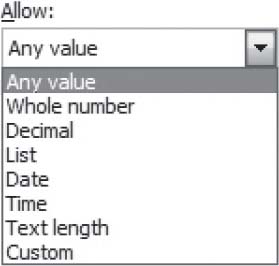
The default setting for all cells in Excel is to allow any value (pictured). This can be changed by changing the selection in the ‘Allow’ drop down box. It may be modified to any of the following:
Most of these criteria do exactly what they say on the tin: by choosing ‘Decimal’, the input must be a number, whereas ‘Whole Number’ allows for integers only. However, making a selection from the ‘Allow’ drop down box is only the first part of the data validation process.
Once a selection has been made (for example, I will use ‘Whole Number’), the dialog box will change appearance, viz.


The ‘Ignore blank’ check box is no longer greyed out. This allows blank cells to be ‘valid’ regardless of the criteria selected. The remainder of the dialog box is governed by the ‘Data’ drop down box. There are various selections that may be made:
Depending upon the choice made, the box will prompt for values (e.g. Minimum and Maximum in the illustration above) which can be typed in, or else the values can refer to cell references directly or indirectly via range names.
One the choices have been made, you might wish to utilise the other two tabs of the Data Validation dialog box.

With the ‘Show input message when cell is selected’ checked, if the end user selects the data validated, cell the message typed in here will appear. This can make data inputs in a model much simpler as end users are ‘spoon fed’ with a pop-up box detailing what to do. In the example below, the ‘Input Restrictions’ comment only appears when the cell is selected:

The third tab selects what to do if invalid data is entered in the cell:
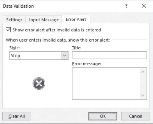
This alerts the end user when an invalid entry has been made (e.g. typing “dog” when a number is expected) - as long as the ‘Show error alert after invalid data is entered’ check box is ticked.
There are three styles available:

The three styles provide differing treatment of invalid data:
•Stop - the value will not be accepted and the end user will be prompted to retry;
•Warning - the end user will be warned that the data is invalid, but be asked whether it is OK to continue; and
•Information - the end user will be advised that the data is invalid but that the data has been accepted.
If the ‘Show error alert after invalid data is entered’ check box is not ticked, no prompt will occur and invalid data will be accepted in the cell without any warning.
Whole Number, Decimal, Date, Time and Text Length are all relatively straightforward, albeit very similar in nature. This leaves just two remaining categories to consider.
This functionality allows the end user to select from a list.

With ‘List’ selected, the dialog box prompts for a source for the list. In the illustration, the entries have been typed in, separated by a comma (the delimiter). However, the data can use cell references which are in a column - or a row - as long as the cells are on the same worksheet in versions of Excel up to and including Excel 2007. This can be limiting and a viable workaround is to name a row or column of data (using the prefix ‘LU_’ for Look Up) and then use the range name here (which may be pasted in using the F3 function key).
For lists, I strongly recommend using the ‘In-cell dropdown’ which provides a dropdown list of valid entries once the cell has been selected.
As you become more experienced, you may find the functionality limiting. This is where the final ‘Allow’ category comes in useful, as you design your own data validation. My recommendation is to experiment with the other types first and then graduate to this classification once you realise validation may not be created using the built-in options.
Data validation will not solve all of your data entry problems. If data has already been entered into a cell and data validation is applied retrospectively such that the contents of the cell would be deemed invalid, no warning will ensue. Similarly, if the contents of a list are altered, any cells that selected the changed value will not update automatically.
To counter these issues, invalid data may be identified on a worksheet as follows:
•On the Data tab of the Ribbon, go to the Data Tools group and click the drop down menu next to the Data Validation icon
•Select ‘Circle Invalid Data ‘ (ALT + A + V + I)

This will circle all invalid data on the worksheet.
One other issue is locating cells that have been data validated in the first place (i.e. no longer allow ‘any value’). The simplest way to do this is through the ‘Go to’ dialog box (F5), click on the ‘Special...’ button and then select ‘Data Validation’ (either all data validated cells on the worksheet or else those validated similarly to the cell(s) presently selected):

Our company produces a monthly newsletter (feel free to subscribe). A short while ago, we polled our readers for their Best Excel Tip ever - and I think it revealed more about the psyche of our average reader than it ever did about improving efficiencies and effectiveness in the workplace...
As discussed above, data validation is a useful way to control what end users can type into a worksheet cell. You can use this functionality to play a trick. Please use this at your own risk: if you get fired, you will get no sympathy here.
If someone is unfortunate to leave a spreadsheet unprotected, simply highlight the whole worksheet and then activate Data Validation (ALT + D + L).
In the ‘Settings’ tab, select settings similar Then, select the ‘Error Alert’ tab: to the following (the aim is to pick a number the user won’t use):
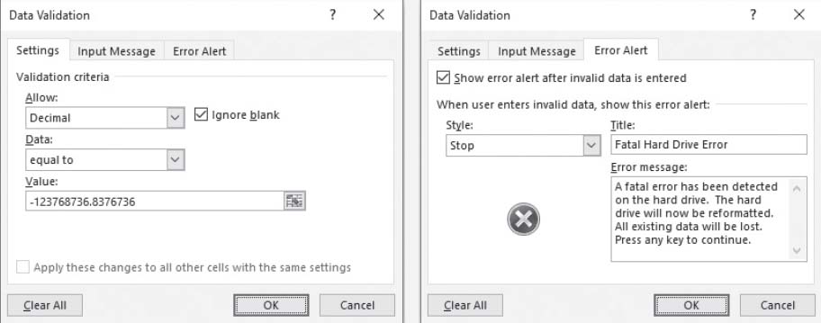
Now, de-select the range and wait for your victim to use the worksheet. As soon as they type an invalid entry, they will be greeted with the following error alert:

Who says spreadsheets can’t be fun..?
The next built-in feature I’d like to address assists with what-if analysis and is an alternative to copy and paste macros. Just to be clear, when I refer to “sensitivity analysis” here, I mean the flexing of one or at most two variables to see how these changes in input affect key outputs. Excel has various built-in features that assist with this type of analysis, but here we will focus on Data Tables.
Data Tables are ideal for executive summaries where you wish to show how changes in a particular input affect a key output. However, as always with modelling, Keep It Simple Stupid (KISS). If you can achieve the same functionality without using Data Tables in a simple, straightforward fashion, then do it that way. Consider the following example:

In this illustration, the key output revenue has been given in cell G11. We want to summarise what happens if we increase (“flex”) this figure by a given percentage, with the inputs specified in cells F17:F26. This can be simply computed by using the formula
=$G$11*(1+$F17)
in cell G17 and simply copying this calculation down.
Data Tables should really be used when such simple calculations are not possible and you want to flex one variable (known as a “one-variable” or “one-dimensional (1-D)” Data Table) or two (known as a “two-variable” or “two-dimensional (2-D)” Data Table).
I will now consider each in turn.
This is best illustrated using the following example.
Now I do appreciate this example could be constructed using a similar technique to our revenue example using the NPV function: I just wanted to construct a slightly more complex alternative that could still be followed!
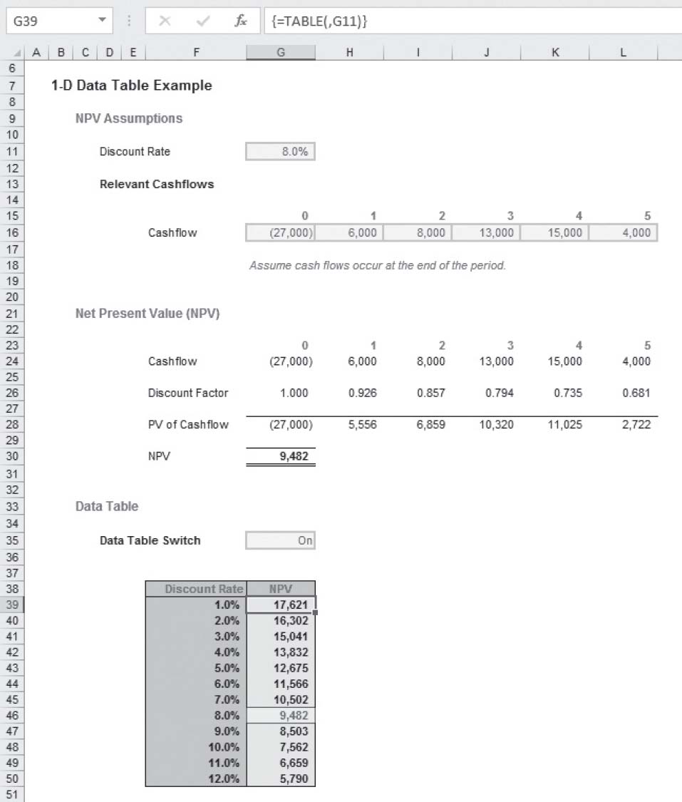
Here, a simple Net Present Value calculation calculated for a total of six periods (0 to 5 inclusive). If you don’t understand what this is, don’t worry, the point is, we are building a calculation. The output for a discount rate of 8.0% (cell G11) is +$9,482 (cell G30). But what if I wanted to know how the NPV would change if I varied the discount rate?
It is very easy to construct a table (a Data Table) similar to the one displayed in cells F38:G50 above. The required discount rates are simply typed into cells F39:F50, but the headings in cells F38:G38 are not what they seem.
For a 1-D Data Table to work using a columnar table similar to the one illustrated, the top row has to contain the reference to output cell in the right hand cell (G38 must be =G30). Many modellers will do this, putting the headings in the row above instead and then they may or may not hide row 38 in order to compensate.
There is a crafty alternative (employed above).
Using CTRL + 1 or ALT + O + E to Format Cells, if we go to the ‘Number’ tab we can still type the formulae in but change the outward appearance of the cell. For example, cell F38 is formatted as follows:

Here, I have typed in “Discount Rate”;”Discount Rate”;”Discount Rate”. Custom number formatting was explained in detail earlier, but essentially this syntax forces Excel to display any numerical output as “Discount Rate”. Note that simply typing “Discount Rate” here once would be insufficient: e.g. if the output were negative, the cell would be displayed as “-Discount Rate”. G38 is formatted similarly.
Once row 38 has been finalised, highlight cells F38:G50 and then create the Data Table as follows:
•Click on the ‘Data’ tab on the Ribbon
•In the ‘Data Tools’ group, click on the ‘What-If Analysis’ icon and select ‘Data Table.” (ALT + D + T or ALT + A + W + T).

This gives rise to the following dialog box:

In a 1-D Data Table only one of these two input cells should be populated. When the table is of a columnar format, the column input cell should be populated, referring to the input cell, as above.
If the table had been across a row instead, ensure that the input values are in the top row, and that the ‘headings’ are in the first column (i.e. transpose the example table above). Then, you would populate the ‘Row input cell:’ box above instead.
Once ‘OK’ has been clicked, the Data Table will populate showing what the NPV would be for alternative discount rates. The formula should be noted: {=TABLE(,G11)} shows this is an array function with G11 as the column input cell. The use of array functions here means that once constructed, the Data Table may not be modified partially.
1-D Data Tables do not need to be simply two columns or two rows. It is entirely possible to display the effects on more than one output at the same time provided you wish to use the same inputs throughout the sensitivity analysis, viz.

These Data Tables are similar in idea: they simply allow for two inputs to be varied at the same time. Let’s extend the 1-D example as follows:

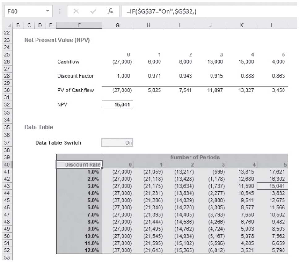
This example is similar, but only calculates the NPV for a certain number of periods - specified in cell G15. Our 2-D Data Table (which is cells F40:L52, not F39:L52) can answer the question, “What is the NPV of our project over x periods with a discount rate of y%?”. It also displays the current value in blue using conditional formatting. Again, if you don’t follow, it doesn’t matter - the point is, there’s a sophisticated calculation here dependent upon two inputs and the output may be summarised easily.
If anything, a 2-D Data Table is simpler than its 1-D counterpart since there is little confusion over row and column input cells. The formula for analysis is always positioned in the top left-hand corner of the Data Table (in this example, this is cell F40). Again, the output needs to be in the table, this time it must be in the top left hand corner of the array. In our example, it is disguised as “Discount Rate” using similar number formatting to that described earlier.
The inputs required now form the remainder of the top row and the first column of the Data Table. With cells F40:L52 highlighted, the Data Table dialog box is opened as before:

Since the top row are the inputs for the Number of Periods, the ‘Row input cell:’ should reference $G$15, whilst the discount rate inputs (‘Column input cell:’) should link to $G$11 once more.
Once ‘OK’ is depressed, the Data Table will populate as required - simple!
Data Tables can be really useful for executive summaries, but there are drawbacks to consider:
•The variable inputs to be flexed should always be hard coded, since formulae may not work as envisaged with this feature. This is due to the fact that these calculations may be dependent upon calculations that may vary for differing inputs, which may change as the Data Table calculates. This can prove cumbersome if you wish to change the Data Tables regularly;
•Data Tables can slow down the file calculation time dramatically. For example, if you have just three 2-D Data Tables, each with ten inputs on each axis, the model calculation time could increase by a factor of up to 300 (= 3 x 10 x 10).
Microsoft has recognised this issue and allows you to change Excel’s Calculation option (found in ALT + T + O, under ‘Calculation’) to ‘Automatic except tables’:

I strongly recommend you do not implement this option. End users tend to assume Excel is always calculating everything automatically and some do not know how to check / modify this functionality.
Instead, I would build in ‘On / Off’ switches next to the Data Tables themselves. These are transparent and intuitive and have the same effect. All that is required is that the output formula is revised to be
=IF(Switch=“On”,Calculation,)
•Data Tables will only flex one or two variables at a time. If more variations are changed, consider using Excel’s Scenario Manager or the Solver add-in (depending upon your requirements, not discussed here);
One other point to note is that although there are workarounds, in general the inputs and outputs should be on the same worksheet as the Data Table. This is not always ideal, but this Excel restriction may be circumvented as follows.
I have a saying that anything is possible in Excel. Maybe one day I may come unstuck, but today is not that day. The issue is that Excel restricts where the referred inputs must be located, i.e. they must be positioned on the same page. If you try and reference cells on another worksheet, or become cunning and use range names which refer to cells on another worksheet (a useful workaround on many occasions), you will encounter the following error message:

Most financial modellers will recall the mantra of keeping inputs separate from calculations separate from outputs. Data Tables force you to put outputs on the same worksheet as the inputs which can confuse end users and make it difficult to put all key outputs together.
So how can you get round this? My solution assumes you do not wish to hide Data Tables on the input sheet and then link them to another worksheet (this is cumbersome and can make the model less efficient).
To make things more “difficult”, I will assume that you have already built your financial model and the Data Tables are to be incorporated as an afterthought. There could be two inputs to incorporate. I will explain how to create one of them (you then just have to follow this process twice).
Firstly, create a “dummy” input cell on the same worksheet as the Data Table. This needs to be protected such that data cannot be entered into this cell. I will assume that this cell is W44 (say) on the Sheet2 worksheet, i.e. the same sheet as the Data Table.

Secondly, link the Data Table (ALT + D + T) to this dummy input (in the illustration here I assume that the Data Table is a 1-dimensional Data Table):

Thirdly, let us assume you want actually want the Data Table to link to “Input 1” (cell D4) on Sheet1:

Fourthly, since we have already built the model this input will already be linked throughout the model. Since I do not wish to change all the dependent formulae, I first cut (NOT copy) the input into an adjacent cell:

Fifthly, a copy is pasted back into the original cell (here, this was cell D4):

Finally, the value in cell E4 is replaced with the following formula
=IF(Sheet2!W44=““,D4,Sheet2!W44)
and then formatted / protected to ensure end users do not actually type into this cell:

The Data Table will now work. This is because:
•The Data Table links directly to a cell on the same sheet as the Data Table, but indirectly to the input on the other worksheet;
•Cell E4 on Sheet1 is now the cell that drives all calculations throughout the model, even though it appears to have been added;
•Cell D4 on Sheet1 still appears to be - and acts like - the original input it replaces.
Three accountants go for a job interview. The first one goes in and is handed a glass of water, precisely half-filled. The interviewer asks him to describe the contents to which he replies, “It’s half empty”. “Thank you,” replies the interviewer, “We will let you know”. The accountant walks out and shrugs his shoulders as he walks past the remaining two candidates.
The second accountant walks in and is asked the same question. She thinks for a second and then responds, “It’s half full”. “Thank you,” replies the interviewer, “We will let you know”. The second accountant walks out. She scratches her head quizzically as she walks away from the final interviewee.
The third accountant - who is also a financial modeller - walks in and is asked the very same question. “What would you like it to be?” the modeller enquires. “When can you start?” asks the interviewer.
Ever since spreadsheets and calculators were invented there have been two types of forecasting task: those that seek accurate forecasting and those that, well, seek the number first thought of. It is commonplace in modelling for users to ascertain what value an input must have in order to achieve a desired outcome. Modellers need to possess the skills to facilitate this even with the most complex spreadsheets. Luckily, there are tools available.
Consider the following example:

Here, let’s imagine we have been asked to calculate the internal rate of return (IRR) on these cash flows (i.e. imagine you could put money in the bank and either invest or pay interest at the same compounding rate. IRR would be the rate which would make the totals including all interest add up to zero).
The Present Value (PV) of a cashflow is defined as “what it is worth today”. Some describe it as compound interest in reverse. If you were to deposit $100 in the bank today at an interest rate of 10% p.a. then in one year’s time it would be worth $110, in two years’ time it would be worth $121 and in three years’ time it would be worth $133.10, etc.
With a discount factor of 10%, the present value of $110 in one year’s time would be $100 today; the present value of $121 in two years’ time would be $100 now; the present value of $133.10 in three years’ time would also be $100 today.
The sum of all present values, both positive and negative is known as the Net Present Value (NPV). Theoretically, if you invest in a project with a particular discount rate - also known as the cost of capital - you should only proceed with the project (from a financial perspective) if the NPV is greater than zero. This is known as value accreting.
The Internal Rate of Return (IRR) is the discount rate which makes the NPV precisely zero.
It will probably not surprise you that I have deliberately chosen a set of values which cause problems for Excel. Excel has two functions which calculate the IRR: IRR (when cashflows occur on a regular / periodic basis) and XIRR (when cashflows do not occur on a regular basis). Neither will work on the above:
•IRR will not work as the periods are not equidistant;
•XIRR gives an incorrect answer (0.00%). If this were correct, then the sum of the cash flows excluding any interest effects (known as the undiscounted cashflows) must equal zero. They do not:

You may have noted that the valuation functions IRR, XIRR, NPV and XNPV have neither been demonstrated nor explained fully anywhere in this book. This is because they do not always calculate correctly. I am a keen advocate of taking these computations back to first principles instead so that everyone may understand how the results have been derived.
So allow me to take this example back to first principles. Here, I have created an elementary Net Present Value calculation:

To generate the value in cell G47, I have manually kept changing it to try to get a zero NPV in cell H59. I did this as follows:
•Typed in a rate of 0%: NPV was $2,325 (positive)
•Tried a higher rate of 10%; NPV was negative, ($6,650)
•Tried a rate of 5% (mid-point between the two rates): NPV was still negative, ($2,666) (still negative)
•Tried a rate of 2.5% (mid-point between 0% and 5%): NPV was ($315) (negative, but getting smaller)
•Tried a rate of 1.25% (mid-point of 0% and 2.5%): NPV was $966 (positive)
•etc.
After a gazillion attempts (look it up, it’s a technical term), I will get very close if I keep bisecting the two rates that provide the smallest positive and smallest negative NPVs. You can imagine this will become heavily time consuming and I will have less time to do the things I would rather do than this - like pulling out my toe nails...
The general rule with financial modelling is whenever you catch yourself doing the same thing over and over again, it’s very likely you haven’t realised there is an easier way to do whatever it is you are doing. Like here. I can use Excel’s Goal Seek functionality to derive the discount rate that will make the NPV zero:

Goal Seek (ALT + T + G, or else go to the ‘Data’ tab on the Ribbon, then in the ‘Data Tools’ group, select ‘What-If Analysis’ and then choose ‘Goal Seek.’) requires three inputs:

The ‘Set cell’ value is the NPV output here, ‘To value’ is the desired outcome (e.g. zero) and ‘By changing cell’ defines the variable input (e.g. discount rate). So what happens if you want to set the ‘To value’ to refer to a cell value rather than a typed-in number?
I have a very simple response: you can’t.
So what can you do instead..?
Excel includes a (hidden) tool called Solver that uses techniques from the operations research to find optimal solutions for all kind of decision problems. It is not situated in the standard loadset: it has to be loaded from Excel’s add-ins.
In any version of Excel, a simple way to access add-ins is to use the keystroke shortcut ALT + T + I:

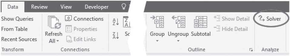
Checking the Solver add-in will add Solver to the ‘Data’ tab of the Ribbon:
Solver is often used to optimise / minimise outputs. Consider the following example:

Imagine you run a company with four products: A, B, C and D. Your intention is to maximise company profits, but you only have 1,000kg of raw material necessary for these four products. If this is all there is to the problem, then it would be simple - only produce Product D. However, imagine you had the following operational constraints:
•For every kilogram of Product B produced, you have to manufacture at least two kilograms of Product A;
•You must produce at least 50kg of Product B;
•Product C is a by-product of Products A and D: the total weight of Products A and D must equal the number of kilograms of Product C produced.
The above graphic shows the optimal solution; the question is, how did I derive it?
To recreate the solution, open the Solver dialog box:

The “objective” here would be the output, i.e. total profit (cell I18 in the example) and the aim is to maximise it (note the other two alternatives of minimisation or trying to generate a particular output value). This is achieved by selecting which cells may be varied (here the kg produced), subject to the constraints specified.
Constraints are simple to include - merely click the ‘Add’ button:

In Excel 2010 and later versions, Solver explicitly allows one of three Solving methods:
•Simplex Method: this method is used for solving linear problems (i.e. where the relationship between variables could be charted using a straight line). Our example above is one such instance;
•GRG Nonlinear: this is used for solving smooth nonlinear problems;
•Evolutionary Solver: this approach uses genetic algorithms to find its solutions. While the Simplex and GRG solvers are used for linear and smooth nonlinear problems, the Evolutionary Solver can be used for any Excel formulas or functions, even when they are not linear or smooth nonlinear. Spreadsheet functions such as IF and VLOOKUP fall into this category.
In summary, Solver is a more powerful variant of Goal Seek, allowing forecasters to derive inputs to achieve specific goals and objectives. However, upon first inspection, Solver still does not appear to allow the value to be set to be a cell reference.
Therefore, you need to employ a simple trick.
In this example, I will return to the NPV example:

In this instance, I could have used Goal Seek as before, but instead I got out the heavy artillery:

The discount rate (Solver_Rate) here is cell G15. You should notice two little tricks though: I have not used the NPV (cell H25) as the output, but a dummy value of cell I19 (the first period’s cash flow). This allows us to select a very useful constraint: that the NPV (cell H25) equals the required value (cell H28). It should also be noted that compounding discount rates is clearly a non-linear calculation technique so Simplex should not be used as a Solving Method.
This has allowed me to show you a neat trick, but I am not entirely convinced of this solution. I cannot help feeling we are cracking a walnut with a thermonuclear warhead and besides, you still have to activate the Solver - this method will not update values automatically as inputs change.
So is there another way..?
Well, yes there is, although it involves VBA, which regular readers will note is a method I try to fall back on when all else fails. This could be argued (perhaps!) as one such instance.

In this example, there are two inputs, initial cash flow and required NPV (cells G15 and H27 respectively). Typing a value in either cell will change the discount rate in cell G13 so that the NPV (cell H25) equals the required value.
This was achieved using a macro.
I have included the macro code by right-clicking on the relevant worksheet tab and select ‘View Code’, viz.

This will launch the Visual Basic Editor:

Not all of the above panes may be visible, but in the right hand pane paste in the following code (as shown in the graphic above):

It is very straightforward: if cell G15 (row 15, column 7) or H27 (row 27, column 8) is edited the macro is invoked and changes the discount rate in cell G13 such that the NPV in cell H25 equals the required output specified in cell H27.
Assuming macros are enabled (see earlier), this will change the discount rate without calling either Goal Seek or Solver. If you choose to use the macro solution, do remember to save the Excel file as a macro enabled workbook!
I commonly use hyperlinks in my Excel files as they are a great way to move around a file. If you create a central worksheet with hyperlinks to all of the other worksheets, you are only ever two clicks away from anywhere else in the workbook. They make life very easy for end users and once you know how to construct them, they take mere seconds to insert.
The ‘Insert Hyperlink’ dialog box is fairly straightforward to use and readily accessed via one of two keyboard shortcuts, either ALT + I + I or CTRL + K. Alternatively, from the Ribbon, select the ‘Insert’ tab, click on ‘Hyperlink’ in the ‘Links’ group:

Hyperlinks can be used to link to a variety of places, but in this instance, I will focus on linking to elsewhere within the same workbook.

To create a hyperlink, first select the cell or range of cells that you wish to act as the hyperlink (i.e. clicking on any of these cells will activate the hyperlink). Then, open the Insert Hyperlink dialog box (above) and select ‘Place in This Document’ as the ‘Link to:’, which will change the appearance of the rest of the dialog box.
Insert the text for the hyperlink in the ‘Text to display:’ input box (clicking on the ‘ScreenTip...’ macro button will allow you to create an informative message in a message box when you hover over the hyperlink).
The next two input boxes, ‘Type the cell reference:’ and ‘Or select a place in this document:’, work in tandem - sort of:
•If you type a cell reference in the first input box without making a selection in the second input box, the hyperlink will link to the cell reference on the current (active) worksheet;
•If you type a cell reference in the first input box and select a worksheet reference in the second box, the hyperlink will link to the specified cell in the given worksheet. In my example above, this hyperlink will jump to Sheet1 cell A1; or
•If you select a ‘Defined Name’ (i.e. a pre-defined range name) in the second input box, this will link to the cell(s) specified. This is the recommended option, where available, if you wish to link to cell(s) on another worksheet within the same workbook. This is because if the destination worksheet’s sheet name were to be changed, the link would still work. I recommend that the range name should start with HL_ for Hyper Link, to make it easier to sort through range names if necessary.
It should be noted that there is an Excel function, HYPERLINK(link_location,[friendly_name]). I tend not to use this as it is not so user-friendly.