In light of the discussion on “Best Practice”, I want to provide some tips on laying out a typical worksheet in a financial model. I want to be clear: no one is holding a gun to your head and saying you must do it this way. I have been modelling for a long time (you’d think I would get the thing finished by now) and I’d like to pass on some of the things I have learned - more often than not, the hard way. I do not profess to be an expert (an “ex” is a has-been and a “spurt” is a drip under pressure). I see myself more as a farmer: a man outstanding in his field (get it?).
So where do I start? Before I start developing a worksheet, let me discuss setting up Excel in the first place. There are ways to make your life a little easier when setting up a spreadsheet - so allow me to set up some of the foundations…
You may have noticed I have been using Excel 2016 screenshots throughout this book. This allows me to stay hip and up to date (my daughter doesn’t agree) and to show off some of the newer features. One such new addition came out in Excel 2013: Quick Analysis.
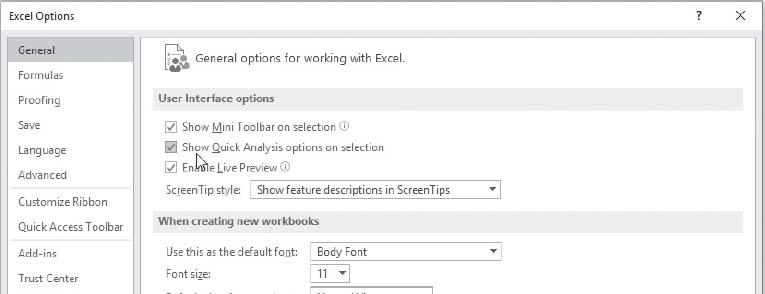
To ensure it is enabled, go to Excel Options (ALT + T + O) and select ‘General’ from the left hand column. Then, ensure ‘Show Quick Analysis options on selection’ from ‘User Interface options’ is ticked:

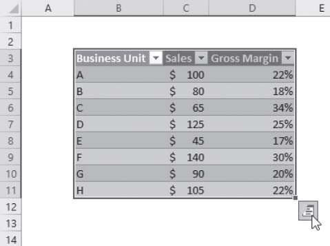
This feature is clearly aimed at those still feeling their way round some of the more sophisticated analytical tools in Excel. All you need to do is highlight the entire data to be analysed (including headings) and click on the Quick Analysis icon in the bottom right-hand corner, viz.

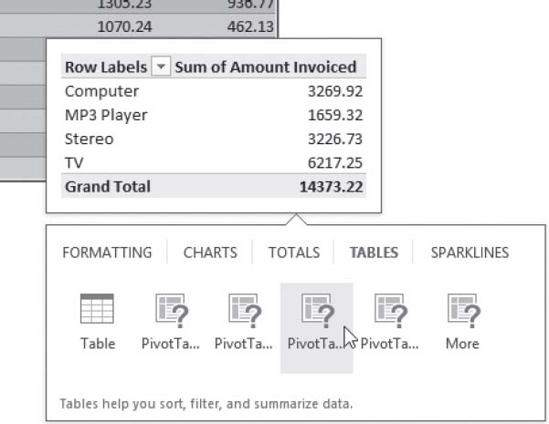
This generates a pop-up menu where the user can make simple selections regarding formatting, charts, totals, Tables, PivotTables and sparklines (charts in a cell). For example:
I recall when Excel 2013 first came out that I ought to be on commission for Microsoft. I used to demonstrate why this tool was so useful by creating a reasonably sophisticated chart with just a couple of clicks of the mouse. In seconds, I used to transform the example:
by clicking on the Quick Analysis tool and converting the data into the following chart:

Now yes, I appreciate it isn’t that difficult to construct that chart. The point I make here is that Excel can create it immediately.
I hate to admit it, but I find as I get older my eyes require longer and longer arms. Finding working on a 75-inch plasma screen a little impractical (and awfully warm!), there is a viable alternative. Go to Excel Options (ALT + T + O) and select ‘General’ from the left hand column. Then, consider the options in ‘When creating new workbooks’:

Changing the font size scales up the workbook fonts including - most importantly - the Formula toolbar. This is particularly useful for tired eyes, presentations and training.
The final option in this section, ‘Include this many sheets’ is also useful if you find yourself copying / deleting worksheets in a newly-created workbook on a regular basis.
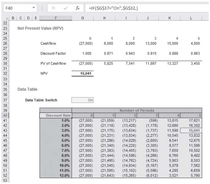
The options in Excel Options (ALT + T + O) -> ‘Formulas’ are useful too.
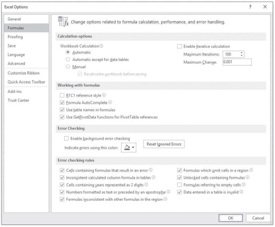
The Workbook Calculation in ‘Calculation options’ should always be set to ‘Automatic’. No exception. Why? Well, how many times have you opened another’s workbook, changed inputs and relied upon the outputs? On those occasions, how often did you check the model calculations were set to ‘Automatic’? Exactly.
There are some professional modelling firms out there that advise you should set calculations to ‘Automatic except for data tables’. Rubbish. Yes, Data Tables may slow a model down, but if you want to a Data Table to cease calculating, it should be done transparently. When I discussed Data Tables earlier, I explained how data validation could be employed to do this on the face of a worksheet, rather than hidden away in Excel Options.
There are other functionalities to consider on this page of Excel Options as well. ‘Formula AutoComplete’ provides the prompt that has made entering calculations simpler since the advent of Excel 2007.

I would recommend keeping that option checked. ‘Use table names in formulas’ and ‘Use GetPivotData functions for PivotTable references’ do similar things. Given Tables and PivotTables may both change structure depending upon filters and the data added, linking to a structured reference such as
=GETPIVOTDATA(“Amount Paid”,$A$1,”Item”,”Stereo”)
can ensure the correct reference is always applied no matter how the structure of the underlying Table or PivotTable may vary.
The last section in ‘Formulas’ concerns error checking. I strongly recommend that ‘Enable background error checking’ is selected. This allows Excel to identify and highlight common errors that modellers make and essentially protects you from yourself.
The options in Excel Options (ALT + T + O) -> ‘Save’ is another area to review.
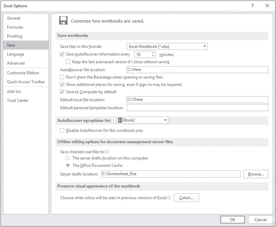
Note the default save format: it is as an Excel Workbook (*.xlsx) file. This type of file does not permit macros. I can understand that Microsoft wants to err on the side of caution and therefore does not allow macros by default, but there are hidden dangers with selecting this option. If you receive an Excel file from a third party and open it, say, from Microsoft Outlook, when you try to save it, Excel will save it as an xlsx file. If there are macros contained within the workbook, these may be consigned to the great macro locker in the sky if the warning message when saving is not read properly. Therefore, it is arguably safer to modify the ‘Save files in this format:’ option to ‘Excel Macro-Enabled Workbook (*.xlsm)’ instead.
The next option down can also be troublesome. For years, scientists have been spending millions on developing AI (Artificial Intelligence). I really do not know why they have bothered. Microsoft perfected this nearly 30 years ago. Ever made a clanger in Excel and you were just about to undo when Excel automatically saved your file?

Microsoft has long since learned when it’s the most inopportune time to save. In the middle of a long, complex formula? Presenting the results to the board? Trying to work out in a rush? No problem, Excel will autosave now, thank you very much. This can be very frustrating - but there is a remedy: either extend the duration or switch it off completely.
Now be careful here. I once recommended this to a group of accountants who the next time they bumped into me had brought along a tree, gallows and a noose. If you switch AutoSave off, make sure you save regularly or you may lose your work. Professional modellers tend to switch AutoSave off but train themselves to save every two to five minutes. Seriously. This way, you can save a file on your own terms.
It is a good idea to have a good nomenclature set up for file saving. I tend to use the format
‘Meaningful Filename vLB1.01’.xlsm
Meaningful Filename is not ‘INT RND OMG FG ex Crs’ or ‘Project Wildebeast’. I am a professional consultant and I have liaised on many confidential projects in my time. Not only have some of the codenames been a mite questionable over the years (‘Project Herpes’ anybody?), but 12 - 24 months later you cannot remember which project goes with which codename. It is better to keep your files in a secure location and call it ‘Chess Pieces Sales Five Year Forecasts’ so you can find it quickly when you need to.
LB simply represents my initials. Don’t use mine, use yours. It’s good to know who the author was as so few modellers bother to update this in File Properties. It gives the end user a fighting chance as to who they ought to approach should they have any queries.
v..1.01 is the version number. Rather than using dates, I use numbering. The date information is stored in the metafile in any case. I tend to add 0.01 to the numbering every two hours. This means that if a file were to corrupt, I never have to do too much rework. It also helps in the consulting industry as I know vLB1.15 represents approximately 30 hours work.
I add 1 to the version number when something significant has happened. This may be to signify that the model has been presented to senior management, or that sales calculations were completely re-worked or that a particular subsidiary’s data has been completely added / removed. These are “landmarks” and it is these changes that should be documented in a File Changes document (I am optimistic that you might be creating one of these!).
Another major source of irritation is trying to save a file for the first time and Excel spends six weeks thinking about it whilst it endeavours to connect to the Cloud. Checking ‘Save to Computer by default’ will save you tearing out all of your hair.
One last item on this page is ‘Disable AutoRecover for this workbook only’. This should not be confused with AutoSave. This is the option whereby Excel will make a valiant attempt to save something of your file should Excel crash so that when you re-open the ‘recovered’ file will be available. It will not overwrite your existing work, but instead create a temporary recovery file for you to inspect and decide whether you wish to retain it.
Now this might seem like switching this option off is like buying a new car without brakes, but if your PC is struggling with memory issues, this may be a reason for considering disabling the option. I vehemently suggest you don’t though: closing other applications down is immensely preferable. It may be better to live without iTunes for an hour or two rather than your friends or family for the weekend…
The largest selection of options in Excel Options (ALT + T + O) is contained in the ‘Advanced’ section. I could probably write a book just going through these options but I think it might be even more boring than this one.
It is worth perusing this section and changing options deciding upon personal preferences. Some of the multitude of options include:
•In ‘Editing options’, you can un-check ‘Allow editing directly in cells’. This will mean all formulae when typed will appear in the Formula bar rather than in the worksheet making it easier to read and easier to select nearby cells with the mouse. Further, with this option unchecked double-clicking on a formula reveals precedent cells (the function F5 will take you back afterwards). This is always the first thing I do in Excel after installing a new edition.
•Checking ‘Enable automatic percent entry’ in the ‘Editing options’ section allows you to type percentages into Excel faster as you do not always have to hunt out the pesky % symbol.
•For those in other regions of the world where the decimal point is replaced by the comma and the comma replaced by the semi-colon for example, it’s possible to change these settings without changing the regional settings on your computer. Simply uncheck ‘Use system separators’ in ‘Editing options’ and make your own choice.
•If you want to access the last few files in the Backstage are of your workbook, check ‘Quickly access this number of Recent Workbooks’ in the ‘Display’ section and specify the number of workbooks you wish to view.
•Sometimes graphics go missing in Excel. No one is quite sure why, but it does happen. To make these objects reappear, go to ‘Display options for this workbook’ and ensure ‘For objects, show:’ is set to ‘All’.
•Don’t want zeros to be displayed? This can be achieved with number formatting (see earlier) or else you can un-check ‘Show a zero in cells that have zero value’ in the ‘Display options for this workbook’ section.
•If you have a more powerful computer and / or you are using 64-bit Excel, you may require a bit more grunt for some of your formulae. In the ‘Formulas’ section, consider checking ‘Enable multi-threaded calculation’ to ensure you are availing yourself of all of your hardware’s capabilities.
•Ever typed ‘Jan’ in one cell, ‘Feb’ in the next cell and then completed the rest of the months by highlighting both cells and using Excel’s AutoFill feature? You are exploiting one of the built-in lists in Excel. If you want to add other lists, it’s easy - simply click on the ‘Edit Custom Lists…’ button in the ‘General’ section and either type the list in manually or link to a pre-existing list in your spreadsheet.
Everyone has favourite features / functions in Excel, some of which are buried away deep in the software. Let me give you an example. Ever closed that final file in Excel 2013 or later version only for the application to close down as well? There is a workaround.
In Excel 2013, simply right-click on the Quick Access Toolbar and select ‘Customize Quick Access Toolbar… viz.

In the subsequent dialog box, select ‘All Commands’ in the ‘Choose commands from’ drop down box and then select ‘Close File’ (with the folder icon, please see the illustration below). Next, click on the ‘Add>>’ button to add it to the Quick Access Toolbar and finally click on ‘OK’ to exit the dialog box.

From now on, simply click on this ‘Close’ icon (Excel 2013 and earlier) / ‘Close File’ icon (Excel 2016) in the Quick Access Toolbar and you will never have to say goodbye to Excel again. In fact, you will see it has its very own keyboard shortcut too: press the ALT button in Excel and it will reveal the number (in the illustration below, it is ALT + 4):

Breaking up can just be so very hard to do!
Right, back to work I suppose. The aim of this chapter is to suggest layout tips for developing your model. To begin with then, here’s something I didn’t prepare earlier:
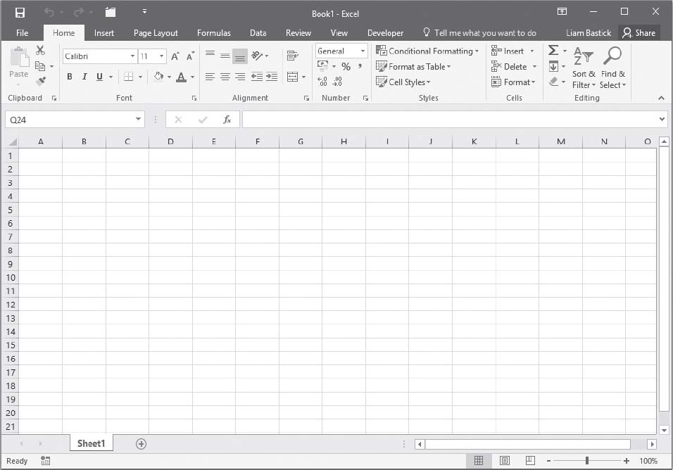
In summary, it’s all about design and scoping. The problem is, we are all time poor in today’s business environment with perpetual pressure on producing results more and more quickly. Getting a layout structure won’t solve all of your problems but it’s a start.
Let me show you how I develop this basic worksheet. Assuming this isn’t a dashboard output page where column widths may be more critical, I tend to narrow the first few columns (highlight columns, then right-click):
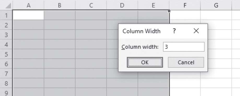
I choose a width of 3 as this effectively makes the cells in these columns square.

You can elect to highlight more or less columns and you can modify the width too. There’s two key points to this:
•Keep column A blank other than for the sheet headings (I will explain later)
•Be consistent, both with the widths of the columns narrowed here and with other worksheets within the same workbook (again, I will explain soon).
Next, let’s put the Sheet Title in cell A1. This should be the same as the description in the sheet tab:
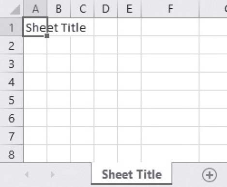
There are three reasons for this:
•Given sheet tab names cannot be infinitely long, sheet titles become more succinct and easier for the end user to understand
•Given the sheet title appears on the worksheet, the name has to be written formally and cannot be an incomprehensible abbreviation, similar to many sheet tab names out there
•This approach promotes consistency, one of the four key concepts of Best Practice modelling.
In cell A2, I will put the model name. This may surprise some of you as this is possible to put in the header or footer of each worksheet instead:
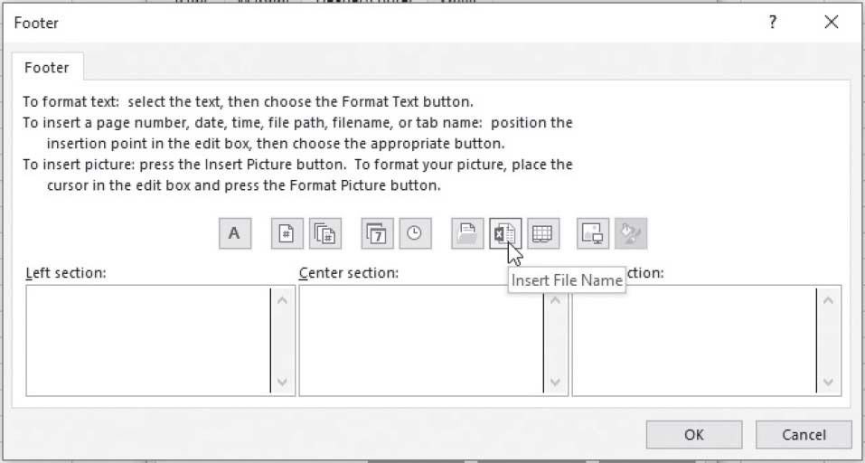
For a start, how many of you know how to locate this dialog box (ALT + P + SP -> ‘Header / Footer’ tab -> ‘Custom Footer…’ button)? This filename will only display when the worksheet is printed. What if it is an image on a PowerPoint slide or, say, as Appendix 4 in a Word document? This is why I keep the model name front and centre on my worksheets.
There’s a formula too:
=IFERROR(MID(CELL(“filename,A1),FIND(”,“(“CELL(“filename”,A1))+1,-FIND(“[“,CELL(“filename”,A1))-FIND),“(“CELL(“filename”,A1))-1)””,

The formula is obvious, yes? I suspect I may need to explain it a little more. It revolves around the CELL function in Excel.
This function returns information about the formatting, location, or contents of the upperleft cell in a reference (in our example, we will be using cell A1 as our reference in the active worksheet, but this selection is entirely arbitrary). The syntax is
CELL(Information_type,[Reference])
and works as follows:
| Information_type Returns | |
| “address” | Reference of the first cell in reference, as text. |
| “col” | Column number of the cell in reference. |
| “color” | 1 if the cell is formatted in colour for negative values; otherwise returns 0 (zero). |
| “contents” | Value of the upper-left cell in reference; not a formula. |
| “filename” | Filename (including full path) of the file that contains reference, as text. Returns empty text (“”) if the worksheet that contains reference has not yet been saved. |
| “format” | Text value corresponding to the number format of the cell. The text values for the various formats are shown in the following table. Returns “-” at the end of the text value if the cell is formatted in colour for negative values. Returns “()” at the end of the text value if the cell is formatted with parentheses for positive or all values. |
| “parentheses” | 1 if the cell is formatted with parentheses for positive or all values; otherwise returns 0. |
| “prefix” | Text value corresponding to the “label prefix” of the cell. Returns single quotation mark (‘) if the cell contains left-aligned text, double quotation mark (“) if the cell contains right-aligned text, caret (^) if the cell contains centred text, backslash (\) if the cell contains fill-aligned text, and empty text (“”) if the cell contains anything else. |
| “protect” | 0 if the cell is not locked, and 1 if the cell is locked. |
| “row” | Row number of the cell in reference. |
| “type” | Text value corresponding to the type of data in the cell. Returns “b” for blank if the cell is empty, “l” for label if the cell contains a text constant, and “v” for value if the cell contains anything else. |
| “width” | Column width of the cell rounded off to an integer. Each unit of column width is equal to the width of one character in the default font size. |
We therefore use the syntax =CELL(“filename”,A1). An example of a returned filename might be:
C:\Documents and Settings\Liam\My Documents\Wretched Book\
Layout Chapter\[Example Layout File.xlsm]Sheet1
This is not what is required, there’s ‘padding’. All we want is the actual filename, in this case ‘Example Layout File.xlsm’. Therefore, we need to extract the filename from this worksheet directory path.
This will be a three-step process.
The directory path will vary for each file, so we need to spot a foolproof method of finding the beginning and the end of the workbook name. Fortunately, Excel assists us here. ‘[’ and ‘]’ are reserved characters in Excel’s syntax and denote the beginning and the end of the workbook name.
The example returned filename above is 105 characters long. If we can find the position of the ‘[’ and ‘]’ we will be on our way.
FIND(find_text,within_text,start_num) is the function we need, where:
•find_text is the text you want to find;
•within_text is the text containing the text you want to find; and
•start_num (which is optional) specifies the character at which to start the search. The first character in within_text is character number 1. If you omit start_num, it is assumed to be 1.
So, in our example, =FIND(“[“,CELL(“filename”,A1)) returns the value 74 and the formula =FIND(“]”,CELL(“filename”,A1)) returns the value 99. In other words, for our illustration, if we can get Excel to return the character string in positions 75 to 99 inclusive (i.e. between the square brackets) we will have our workbook name.
There are various functions in Excel that will return part of a character string:
•LEFT(Text,Num_characters) returns the first few characters of a string depending upon the number specified (Num_characters). This is not useful here as we do not want the first few characters of our text string;
•RIGHT(Text,Num_characters) returns the last few characters of a string depending upon the number specified (Num_characters). This is not useful here either as we do not want the last few characters of our text string; and
•MID(Text,Start_num,Num_characters) returns a specific number of characters from a text string, starting at the position specified, based on the number of characters chosen.
Therefore, we should use the MID function here. In hard code form, our formula would be:
=MID(CELL(“filename”,A1),75,24)
where:
•75 = position one character to the right of ‘[’ (74 + 1); and
•24 which is the length of the filename string, being the position of ‘]’ less the position of ‘[’ less 1, i.e. 99 - 74 - 1 = 24.
This gives us our filename ‘Example Layout File.xlsm’.
The problem is we don’t want hard code: a flexible formula is required. Using the concepts explained above, we derive:
=MID(CELL(“filename”,A1),FIND(“[“,CELL(“filename”,A1))+1,FIND(“]”,
CELL(“filename”,A1))-FIND(“[“,CELL(“filename”,A1))-1)
And so we are done. Except we aren’t.
A good modeller will always ensure that a formula will work in all foreseeable circumstances. The above formula will only work if the file has been named and saved. Otherwise, CELL(“filename”,A1) will return empty text (“”), which will cause the embedded FIND formulae to return #VALUE! errors, and hence the overall formula will also return the #VALUE! error.
We therefore need an error trap, i.e. a check that ensures if the file has not yet been saved we just get empty text (“”) returned. To do this, we can use the following formula:
=IFERROR(MID(CELL(“filename”,A1),FIND(“[“,CELL(“filename”,A1))+1,FIND(“]”,CELL(“filename”,A1))-FIND(“[“,CELL(“filename”,A1))-1),””)
IFERROR(Formula,Error_trap) has been discussed earlier and prevents the #VALUE! error. It isn’t pretty, it’s not short, it’s not transparent, but it’s flexible and robust.
The formula above is intended to be copied - as is - straight into an Excel worksheet by pasting it directly into the Excel formula bar and pressing ENTER. In certain situations, it will not work due to the exact method of copying employed, fonts used or the set-up of the ASCII characters.
In this instance, try re-typing all of the inverted commas (“ and ”) in the formulae first. If that doesn’t work, I apologise, but you will have to re-type it. C’est la vie.
You have to admit that is quite a comprehensive example. Assuming you are still awake, we can employ a very similar formula to the Sheet Title in cell A1:
=IFERROR(RIGHT(CELL(“filename”,A1),
LEN(CELL(“filename”,A1))-FIND(“]”,CELL(“filename”,A1))),””)

The aim is to automate as much as possible. It may not adhere to the “Rule of Thumb”, but sometimes, you have to balance transparency against flexibility and robustness.
20,000 pages into this chapter and I am about to consider what to put on Row 3.

It looks like I have added a hyperlink in cell A3, right? Not quite. I am a little craftier than that. Actually, I have highlighted cells A3:F3 and then merged the cells using Excel’s Merge Across functionality (ALT + H + M + A):

I have discussed how to create hyperlinks earlier in the book (CTRL + K). The intention is to set up a central Table of Contents worksheet where all of the hyperlinks to the other worksheets reside:
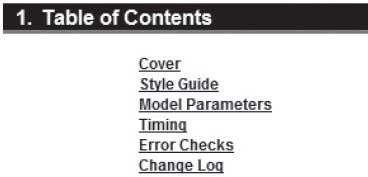
The hyperlink should link to cell A1 of that worksheet and that cell should have a range name such HL_TOC for reasons explained previously. The reason cells A3:F3 are merged is so that if the end user clicks anywhere in that range the hyperlink will activate; otherwise, the user will have to click on cell A3 only for the hyperlink to work.
This brings us on nicely to cell A4:
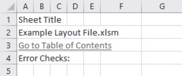
Not much to say about typing text into cell A4, but there is more to do on this row:

Cell F4 is not just the word “OK”; it actually links back to an Error Checks worksheet. I am going to talk about constructing error checks in a subsequent chapter, so imagine for the moment that cell F4 is a formula to another worksheet. In reality, it will also be a hyperlink, but as I said, more anon.
In my layout, I have made column G my Units column: down this column I shall put in all of my units so end users may distinguish between numerical fields. How often have you seen an output and not known if it is in $, $’000, $m, kg or sliced dolphins? This will make this issue a thing of the past. It should be noted that this column is not always required. For instance, on an outputs worksheet, you may simply state near the top of the sheet, “All outputs are displayed in $m unless stated otherwise”.
Cells J4:N4 contain the date headings. In the next chapter, I will explain that you actually need more than one row of details for the dates, but that can keep for now. The dates should be periodic (e.g. monthly, quarterly, annually) and should always start and end in the same columns (and rows) on each forecast worksheet. That is not always possible: sometimes, you require some parts of your model to be annually forecast and other aspects monthly. Where this occurs, this should be in clearly delineated areas of the workbook.
Certainly, under no circumstances should the periodicity be inconsistent across any row of an input or calculations worksheet. It is foreseeable that an output sheet may summarise differently, but this should use a methodology such as SUMIF or SUMIFS (see earlier) to summarise data from other worksheets where the periodicity was consistent throughout, e.g.

You may have noticed as well that there is a line inserted in between rows 4 and 5 of our image:

This is not a drawn line. This is a frozen pane. Frozen panes break up the worksheet in to as many four pieces. Located in the ‘Window’ grouping of the ‘View’ tab of the Ribbon, there are three ways to create a frozen pane:
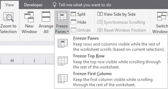
•Freeze top row: Keeps the top row visible no matter how far down the spreadsheet you scroll
•Freeze first column: Keeps the first column visible no matter how far to the right you scroll the spreadsheet
•Custom (Freeze Panes): Creates a frozen locus at the intersection of the top row and the first column of the cell(s) selected.
That final option is a little confusing. Essentially the frozen panes are created as follows:
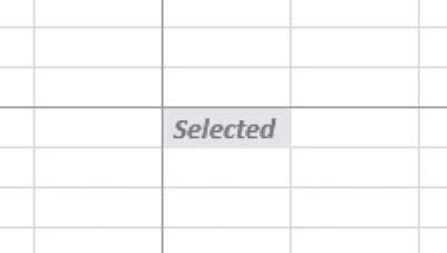
Frozen panes are created for the region the selection is in, the region directly above, the region to the immediate left and diagonally opposite the top left hand corner of the selection. If the selection were in column A, there would only be two frozen panes: the rows immediately above and the remainder. If the selection were in row 1, again, there would only be two frozen panes: the columns to the left and the remainder.
Splits are similar to frozen panes. They are created like Freeze Panes (keyboard shortcut: ALT + W + S). but create scrollbars in all quadrants, which means no section is truly fixed.
In our example, cell A5 has been made the basis of the frozen pane, so that rows 1 to 4 will always be visible. This cell should be given a range name, e.g. HL_Home, as this is the cell hyperlinks to this sheet should link. This cell ‘resets’ the sheet and makes the model easier to navigate as a consequence.
The cell that effectively resets the worksheet can be readily identified. If there is a split or frozen pane on the worksheet, then the chances are cell A1 is not the correct cell. The cell can be identified by the keyboard shortcut CTRL + HOME. It is always the top left hand corner of the bottom right hand quadrant of any frozen panes. It is the top left hand corner cell of the range selected to freeze panes in the first place.
Back to our example, headings should start in column B, not A, and then move out a column or two for sub headings and sub sub headings respectively. I then put data labels directly beneath sub sub headings:

I have called them “Headings” and “Sub Headings” etc. to make it clear, but if I develop a stutter I might be in column Q before you know it! Renaming the headings “Heading 1” and so on may be clearer. This also makes them consistent with pre-existing Style names (hint, hint):

Aside from keeping column A clear, do you now see why I have narrowed columns B, C and D (I am keeping column E “just in case”)? The narrowing of the columns effectively indents the headings and makes worksheets easier to read and navigate (especially if the gridlines, ALT + W + VG, are toggled off).
Take special note of the spacing: one blank row between headings; two lines between sections. That’s my preference. You choose your own if you would prefer - just be consistent. This treatment will reap dividend as our financial model case study later will demonstrate.
Blank columns H and I are in existence in case we have any calculations, inputs or referred values that do not refer to a particular time period. If they are not required, I tend to narrow the columns to a width of 1 (say), so that they are still there in case they are needed later.
Adding labels, data and formulae:
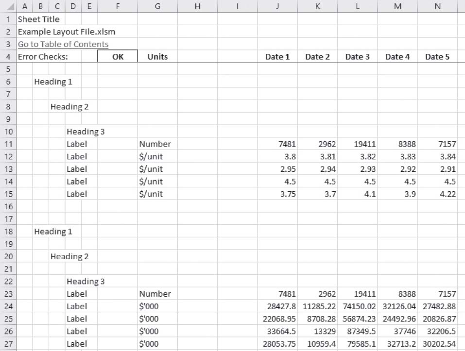
It’s starting to look more like a spreadsheet now. If we start adding / taking into account Styles (ALT + H + J),

these may be applied:
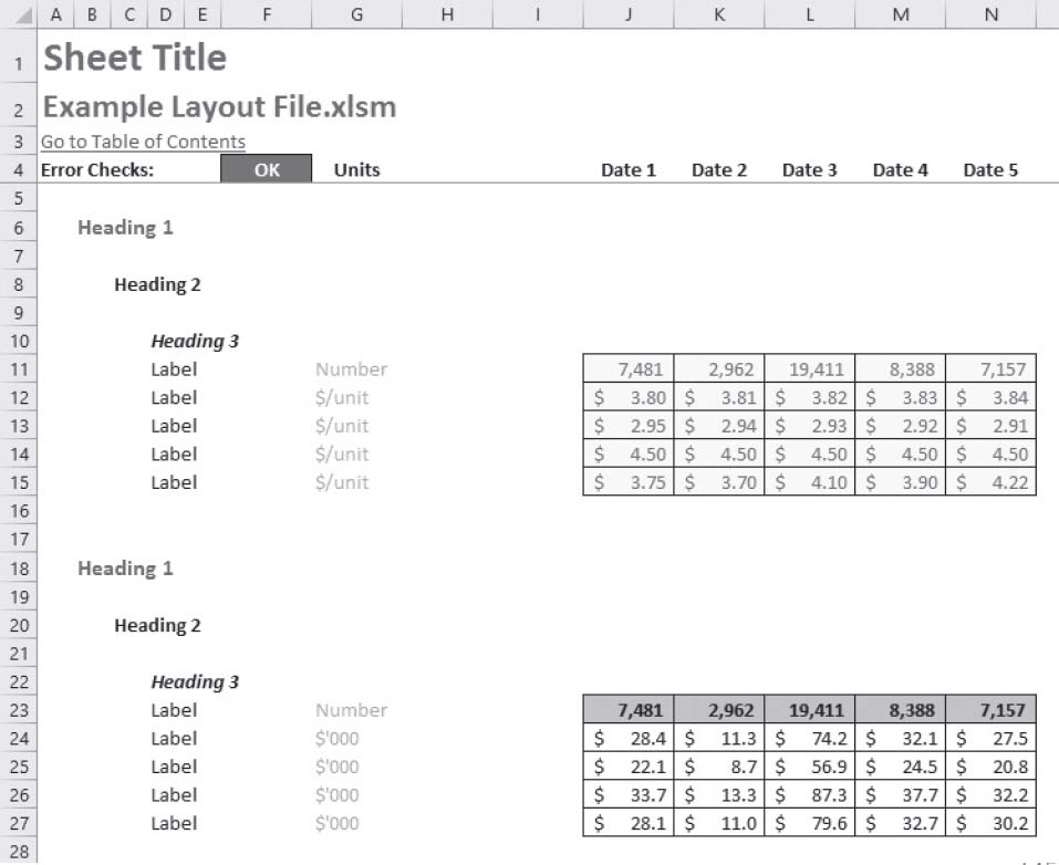
Do you see? It’s starting to look more like a spreadsheet already. I switch off gridlines on my spreadsheets so that the majority of my files appear to have a white background. There is more to this point than merely aesthetics. Adding a colour to the background of a spreadsheet can make a file significantly larger - unnecessarily.
The spacing is deliberate too. Not only does it look neater (remember, Excel 2007 onwards has 1,048,576 rows and 16,384 columns, i.e. it is 1,024 times larger than an Excel 2003 worksheet so there is plenty of room), but the space is functional too.
Want to navigate between the main headings in column B? Click on cell B6, go CTRL + Down Arrow and you will arrive at cell B18. Repeat this action and the next cell you will hit is cell B1048576, i.e. the very bottom of the spreadsheet because there is nothing else in this column.
Click on cell D10 (Heading 3) and go CTRL + Down Arrow will take you to cell D15, the final cell in the contiguous range. CTRL + Up Arrow, CTRL + Right Arrow and CTRL + Left Arrow will all perform similar actions. Need to highlight a range? Click on any cell within the range and CTRL + A will select the whole contiguous range. This makes the model easier for developer and user alike to navigate and manipulate.
So why have I kept column A blank? The reason is to take into account work in progress. How often have you started creating a spreadsheet only to be interrupted, have to go to a meeting, take a telephone call, go home or go to sleep? The point is, when we are interrupted we need to remember how far along we were. If you design a spreadsheet similar to the one discussed here, imagine you are interrupted without notice. Before you turn your attention to the disruption, whichever row you are working on, press the HOME key which will take you to column A of that row. Type anything in that cell, e.g. “w” for “work in progress” or “check” and so on. That’s it.
How does that help you? Before you hand the model to anyone else, we need to undertake some checks before saving and distributing. One of those checks will be to ensure there is nothing in column A of any worksheet after the frozen pane. I will explain how to do this when we discuss reviewing the model at the end of this book. I bet you can’t wait…
That’s all I wanted to say about layout. Keep it consistent, make it transparent, ensure there are checks to protect the robustness and that inputs are clearly marked to aid flexibility. See? I have developed a simple layout adhering to the CRaFT methodology.