But nothing, from mushrooms to a scientific dependence, can be discovered without looking and trying.
—Dmitry Ivanovich Mendeleev, 1834–1907, creator of the first periodic table
From Principles of Chemistry, Vol. 2 (1905)
It is a capital mistake to theorize before one has data.
—Sherlock Holmes, fictional detective created by Sir Arthur Conan Doyle in the late nineteenth century
From the short story “A Scandal in Bohemia” (1891)
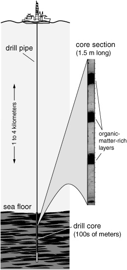
Though the concept of the biomarker emerged from attempts to infer the provenance of petroleum and the incidence of life on the young earth—for all the successes and disappointments of the early studies on Precambrian rocks, lunar dust, and oil shales—it was in the sediments of the deep sea that biomarkers really came into their own. The Deep Sea Drilling Project (DSDP) was initiated in the 1960s by a consortium of American oceanographic research institutions, but institutions in Russia, the United Kingdom, France, and Germany were quick to sign on. In what began as an effort to understand the makeup and dynamics of the earth’s crust and mantle, the DSDP’s special research ship traveled the world’s oceans, drilling thousands of meters into the seafloor to retrieve sediment cores that soon became coveted objects of study for geologists, oceanographers, biologists, paleontologists, and geochemists around the world.
When Geoff’s group started analyzing the DSDP sediments in the early 1970s, most of the organic chemists involved with the program were from the oil industry and formed part of the drill ship’s safety program, monitoring the cores as they were brought on deck to ensure that dangerous accumulations of gas or liquid hydrocarbons weren’t being penetrated. But Geoff saw the DSDP as the perfect opportunity to wean his Bristol lab of its dependence on NASA’s Apollo program—a chance to bring his full attention back to Earth and its still largely unexplored realm of fossil molecules. The British Natural Environment Research Council had earmarked a large pot of funding for work on the cores, which would be unencumbered by the narrow commercial goals and secrecy that surrounded the limited offerings from oil-company bore holes. Geoff’s budding Organic Geochemistry Unit would be aligned with a multidisciplinary community of scientists who were all studying the same cores, working cooperatively, and publishing freely. And, unlike the lunar samples, ocean sediments were rife with interesting organic compounds, including many entirely unforeseen structures. Most of the cores consisted of sediments that had been laid down and buried sequentially without ever being subjected to the tectonic turmoil of stretching and subsidence, and the overlying kilometers of cold water had kept their temperatures relatively low. The result was that many of these organic structures were phenomenally well preserved, with vestiges of some of their biological functional groups persisting for millions, sometimes even tens of millions, of years. Here was an even better sequential record of diagenesis and the progressive fossilization of biological organic molecules than either the Messel or Green River shales could provide. Eventually, as the DSDP ship set out on ever more expansive drilling expeditions, its cores would also provide a record of almost every imaginable marine environment to have graced the earth in the last 150 million years of its history.
The grand majority of the organic matter formed in the ocean comes from microscopic algae, zooplankton, and microbes, and yet knowledge of the chemistry of such organisms was limited. Many of the compounds the geochemists found in surface sediments had never before been identified in organisms. When Geoff and his cohorts first started analyzing the DSDP cores, their biggest task was to identify as many of these new compounds as they could, an endeavor that the geologists who were running the show viewed with some disdain. The geologists had just had huge success with a more hypothesis-driven breed of science, having found evidence for the theory of seafloor spreading and continental drift during the drill ship’s first transect of the mid-Atlantic ridge, precisely where they had predicted it. Geoff recalls that one of them accused him of “just stamp collecting,” an insult that gets him riled up to this day. After all, geologists had spent more than a century obsessively identifying and classifying minerals, rock types, and fossils, whereas the organic geochemists had only recently begun their surveys—though there’s no denying that they were obsessed with their molecular finds. Geochemists in the Strasbourg and Bristol labs, and in Jan de Leeuw’s group in the Netherlands, and even Jürgen working in Dietrich Welte’s petroleum-oriented group in Jülich, all gleefully indulged their passion and made a fine art of determining the precise structures of the compounds they found in marine sediments, as well as lake sediments, microbial mats, and any other promising detritus they could get their hands on. The natural history of molecules was still in its infancy, and there were vast, virgin territories yet to be explored. But the grand attraction of the sediment cores from the drilling project was that they provided both a chemical chronicle of the last 150 million years of earth history and a lesson in how to read it. Despite the geologists’ disdain, the geochemists with their molecule collecting were in no way divorced from the DSDP’s lofty goals of understanding the history of the earth and its climate and life—they just thought it might be a good idea if they learned how to read before attempting to write a magnum opus.
The layers of sediment in the DSDP cores were dated by interdisciplinary teams of scientists using everything from the slow decay of naturally occurring radioactive elements in minerals to the changing assemblages of microfossils. Thousands of meters and hundreds of millions of years of ocean sediment can accumulate without ever reaching more than 50–60°C, temperatures that are generally too low to break down the insoluble kerogen and release hydrocarbons into the bitumen. It was thus possible to observe the various intermediate compounds in the low-temperature stepwise conversion from reactive biological compounds to stable molecular fossils by analyzing the soluble organic matter of the sediments, without having to consider the largely unfathomable processes occurring within the solid matrix of the kerogen.
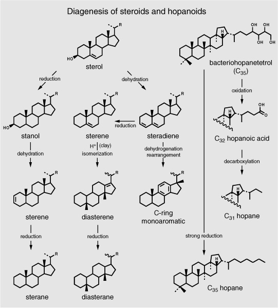
Most of the organic material that forms in the surface waters of the ocean is recycled there; of the 1–2% that does reach the seafloor, more than 90% is usually burned for energy by bacteria in the top few centimeters of the sediments, and much of the remainder is bound up in the insoluble protokerogen. By the mid-1970s, a number of organic chemists at Woods Hole Oceanographic Institution in Massachusetts were following Max Blumer’s lead, tracking the fate of specific organic compounds from marine organisms to the sediments and trying to determine what happened in the water column—what compounds were recycled and what survived to reach the sediments. In keeping with what the Bristol, Strasbourg, and Dutch groups were finding in lake sediments, the tiny proportion of the organic matter generated by phytoplankton in the surface waters that persisted in the sediments and eluded incorporation into the insoluble kerogen consisted mostly of pigments and the lipid components of cell membranes: chlorophyll and carotenoids, fatty acids and alcohols, acyclic isoprenoids, sterols, and hopanoids. In the DSDP cores, the loss of oxygen-containing functional groups and reduction of these biological molecules—decarboxylation of acids, dehydration of alcohols, hydrogenation of double bonds—to their bare carbon and hydrogen skeletons proceeded so slowly that one could work from the surface sediments downward into ever more ancient sediments and infer the progress, step by step. These long, coherent sequences of immature marine sediments contained actual evidence of chemical and microbial transformations that geochemists had hitherto only been able to theorize about.
The Bristol group immediately set about trying to follow the convoluted fate of the sterols produced by organisms. And James Maxwell, of course, looked for the intermediates in the hypothesized transformation of chlorophyll—phytol being oxidized or reduced to pristenic acid and phytenes, and eventually to pristane and phytane, and the chlorin hearts that were gradually aromatized and transformed to the blood-red porphyrins found in oil and ancient rocks. Jürgen says he got involved with the DSDP in the 1970s because Germany, as a new member of the international consortium, had been asked to assign an organic geochemist for one of the cruises and a colleague in the Jülich lab was drafted for the task. The colleague, a geologist and organic petrographer, found the cores so interesting that he put in requests for samples from future cruises and convinced Jürgen to analyze them on the GC-MS—but then quit the lab to pursue other endeavors. Jürgen was left with what seemed to be a relentless supply of DSDP samples to analyze and report on, a task that at first seemed rather pointless. But it wasn’t long before he was thoroughly addicted and clamoring for more; the samples were a treasure trove of new natural products and structure identification challenges, not to mention a virtual connect-the-dots picture of diagenesis. Despite a lack of interest on the part of the petroleum companies that the Jülich institute was supposed to cater to, he convinced Welte to continue the work with the DSDP cores.
As the sediments aged, there were systematic trends in the relative abundances and nature of the compound classes. Short-chain and unsaturated fatty acids in the soluble organic matter disappeared first, either consumed by bacteria or incorporated into the kerogen; likewise, most alcohols and ketones disappeared rapidly, giving way to alkenes and alkanes. The sterols made by organisms lost their hydroxyl groups in a dehydration reaction, and the resulting sterenes, with two double bonds, underwent a complex array of rearrangements and then could be reduced to steranes or, in certain kinds of acidic sediments, to diasteranes, or somehow oxidized to monoaromatic steroids. The A- and B-ring monoaromatics appeared in early diagenesis, but then disappeared, their fate unknown, whereas the C-ring monoaromatics showed up in late diagenesis and survived for hundreds of millions of years, and the triaromatics didn’t appear at all in most of the relatively low-temperature marine sediments. In keeping with Guy Ourisson’s and Pierre Albrecht’s petroleum studies and their observations from modern lake sediments, bacteriohopanetetrol produced by the bacteria in the surface sediments underwent analogous defunctionalization, this time with accompanying degradation of the side chain containing the hydroxyl groups and stereochemical isomerization at the 17 and 21 positions of the pentacyclic structures. And, as Jaap Sinninghe Damsté and de Leeuw would discover in the 1980s, at some point quite early in this process, the double bonds in alkenes and sterols and carbonyl groups in ketones reacted with dissolved sulfide compounds in the sediment pore waters to produce a plethora of organic sulfur compounds.
How fast and to what extent these transformations occurred seemed to depend strongly on conditions in the water column and sediments at the time of deposition. Within a hundred thousand years in a typical deep-sea sediment—pale gray or white limestone and mudstones containing less than 1% organic matter—the fatty acids had been radically depleted and transformed, most of the alcohols had lost their hydroxyl groups, and alkenes and reduced alkanes ruled the day. But in some sediments where rapid burial and a low oxygen concentration had conspired to preserve the organic matter from decomposition—places where upwelling of deep water resupplied nutrients at the surface and productivity was high, or along continental shelves where rivers had deposited a lot of refractory organic matter from land plants—sterols, saturated fatty acids, and long-chain alcohols could persist for more than 10 million years.
Whereas kerogen still stood like an impenetrable knowledge blockade between the molecular fossils in mature rocks or petroleum and their sources, the emerging understanding of diagenesis made it possible, at least in principle, to link many of the compounds found in ancient ocean sediments with the specific organisms or groups of organisms they came from. In some cases, biogenic lipids replete with their double bonds and oxygen-containing functional groups could be found in ocean sediments that were laid down millions of years ago, which was almost like finding a dinosaur bone with some organs or pieces of muscle still attached. Even so, it was no easy task to link a compound found in the sediments, even recent sediments, to the organism or group of organisms that made it—and ultimately, it was this connection that would allow the molecule collectors to read a history of life that was invisible to the geologists, climatologists, biologists, and paleontologists. Despite their collector’s mania, these were, after all, chemists with a sense of adventure, refugees from the tedium of synthetic chemistry and veterans of the search for natural products who were intent on exploring the interface between organisms and their environment through geologic time.
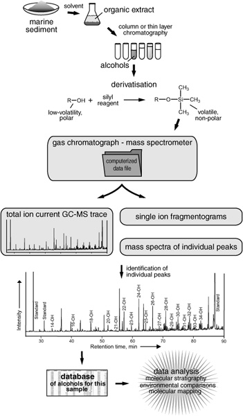
They used the same basic extraction and separation techniques that Geoff and Al Burlingame had started using in Melvin Calvin’s lab in Berkeley, procedures that had been refined to perfection for the first Apollo samples: extract all the soluble organic compounds from the sediment into some solvent mixture such as methanol/chloroform, pour the mixture onto a chromatography column or thin-layer plate to separate them into groups of different polarity—nonpolar hydrocarbons, then aromatics, esters, ketones, alcohols, and so forth—and run each fraction on the GC-MS to separate and, with any luck, determine the structures of some of the hundreds of compounds it contained. When Sinninghe Damsté and de Leeuw began to realize how much information was hidden away and protected in the sulfur compounds, they added desulfurization and other steps that allowed them to separate and analyze the full array of sulfur components. But the basic extraction and separation scheme used for the DSDP sediments in the 1970s and 1980s was not hugely different from that developed in the 1960s and, for that matter, the one used by organic geochemists to this day.
In the 1970s, the so-called molecule collectors looked for suites of compounds that might be biosynthetically related or linked through diagenesis: acids, alcohols and ketones with similar chain lengths, or sterols, sterenes, and steranes with the same side chains. They focused on the most plentiful compounds partly because these were the easiest to analyze, and partly because they promised to come from some prominent member of the ecosystem. And they focused on the most unusual structures, not only because they were the most fun to figure out, but also because they were likely to contain more specific information about the organism or process that made them. Occasionally, they got lucky and the association between compound and organism was readily apparent.
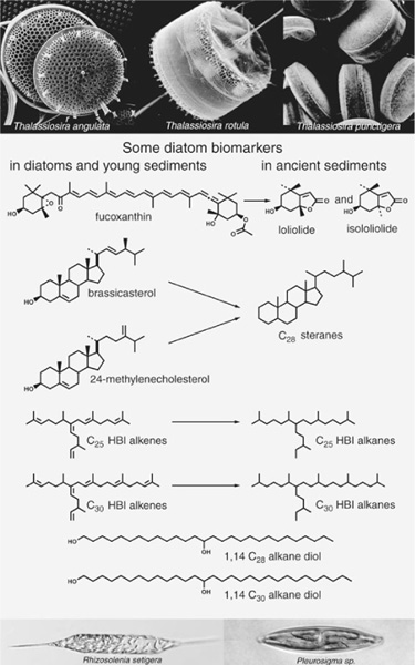
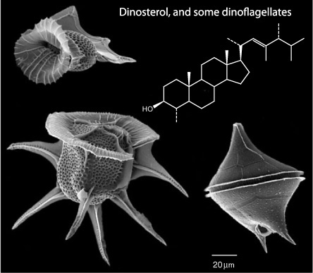
Though it was the mystery of kerogen that had initially inspired de Leeuw, the soluble organic matter in freshly deposited surface sediments obviously held some clues about what had gone into its making and, as it turned out, offered more immediate gratification than the recalcitrant kerogen. Here, at least, one could have the satisfaction of proving a new chemical structure, not to mention lots of publications and successful Ph.D. theses. It wasn’t long before de Leeuw had hooked up with Burlingame’s state-of-the-art analytical laboratory, gained access to samples from DSDP cores, and earned his Dutch group a reputation as a bastion of first-class molecule collectors. One of its first big successes came, however, not from the long deep-sea cores, but from a 5,000-year-old layer of surface sediments in the Black Sea. Here the group found massive amounts of a sterol with a “peculiar” structure, similar to one that had puzzled the Strasbourg group when they identified it in the Messel shale a few years earlier. The Black Sea sediments, however, were also loaded with the distinctive fossils of dinoflagellates, a large, diverse genus of single-celled algae, and the Dutch group suspected this was the source of the sterol. In 1978, around the same time they determined its structure, a group of Rhode Island natural products chemists who were studying the toxin-producing algae responsible for the deadly “red tides” that periodically occur in coastal waters began isolating sterols from dinoflagellates and confirmed de Leeuw’s suspicions: the most prevalent of the sterols, which they christened dinosterol, was none other than the Black Sea sterol, a hitherto unknown structure, with a methyl group attached to the A-ring, and an extra branch attached to its side chain.
Molecular analysis of immature marine sediments (one example: alcohols)
Dinoflagellates are known to paleontologists from the cysts they form during dormant periods, which had allowed them to distinguish hundreds of living and extinct species. These are made of a resistant organic polymer that is readily fossilized and can maintain its distinctive shape and decorations for millions of years, but the organisms only make them when they go dormant, and many species of dinoflagellates don’t make them at all. Most of them do, however, make dinosterol. Once it had been identified, geochemists were able to detect it or its diagenetic successors in sediment cores dating back hundreds of millions of years. Sterols with the same or similar skeletons have been found in small amounts in a few other microorganisms, but 25 years’ worth of research has confirmed that concentrations of dinosterol in sediments generally depend on dinoflagellate populations. It can be used to track the periodic bursts of dinoflagellate productivity in surface waters, providing valuable insight into how the ecology of a lake or coastal marine environment has changed over time. Petroleum geochemists use the presence of dinosterane in petroleum source rocks to provide information about the environment where they were first deposited, and environmental scientists measure the content of dinosterol in the sediments of lakes and estuaries as a way of gauging nutrient inputs and tracking the effects of fertilizer use and runoff in a region.
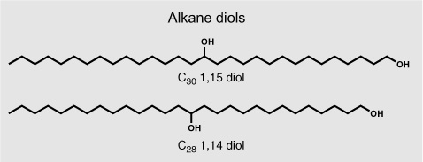
Few of the thousands of compounds identified in sediments during the 1970s and 1980s were as readily linked to a specific class of organisms as dinosterol. Many were constituents of a broad range of organisms and too general to provide much information. Others, like the extended hopanoids, had never been identified in organisms at all, and it took a fortuitous mix of experience, insight, and luck to find their biological parents. A series of long-chain alcohols that the Dutch group found in its Black Sea cores in the 1970s would remain orphans for more than 20 years. These alkane diols constitute a homologous series of simple n-alkyl chains with 28–32 carbon atoms, slightly glorified by two hydroxyl groups, one on the first carbon, and a second in the middle of the chain at C-14 or -15. They turned up regularly in surface and ancient marine sediments from all over the world, but neither they nor any plausible precursor molecules could be found in organisms—not that most natural products chemists were really looking for such compounds.
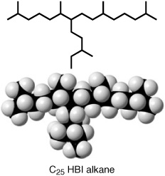
A series of somewhat more distinctive compounds, also noted in the sediments in the mid-1970s, were so difficult to separate from the mixtures of branched and cyclic hydrocarbons that it was years before anyone determined the precise structure of their carbon skeletons. Dubbed “highly branched isoprenoids” or HBIs, they are composed of a saturated or unsaturated isoprenoid chain with another branching from its middle in an odd T-shape. James Maxwell and one of his students first determined the precise structure of a 20-carbon HBI alkane in a sediment extract in 1981, but despite the near ubiquity of such compounds in marine and lake sediments—and, as it turns out, some pharmaceutical potential—another 10 years went by before a source of HBIs was identified in marine organisms.
Highly branched isoprenoid (HBI)
Another series of compounds that the Dutch group identified in sediments from an Atlantic DSDP core in 1978 took only a few years to trace, but this required a complex coincidence of international encounters and interdisciplinary collusion. Indeed, if it hadn’t been for a few worried Scottish fishermen with a lemonade bottle in the North Sea, the most useful and powerful biomarker to date might well have languished among the molecular orphans with the alkane diols for years to come.
In the spring of 1975, amid concerns about the local fishing industry, British Petroleum installed the first of its Forties oil field production rigs off the coast of Scotland. A few days later, when a small commercial fishing boat sailed into an expanse of eerily opaque white water in the normally dark-blue North Sea, the fishermen were convinced that it was pollution from the oil production rig. They filled a lemonade bottle with the milky water, which extended for hundreds of kilometers, and when they returned to shore they delivered the sample to the Aberdeen Marine Laboratory. From there, it made its way around the area’s research labs, and eventually, when no one could detect any petroleum hydrocarbons, it ended up on biochemist John Sargent’s desk.
Sargent was a specialist in the lipids of marine organisms, particularly in the fats and long-chain esters, or wax esters, used for energy storage in zooplankton. When he analyzed the milky water, he found it was loaded with wax esters from copepods, the tiny shrimplike crustaceans that feed on microscopic algae and bacteria. He figured that there must have been a copepod population explosion in the area and their waxes had made the water look milky. He’d observed a similar phenomenon in British Columbia a few years before, when the die-out of a big population of copepods had left the beaches literally covered with sticky wax. But a colleague suggested that the wax esters might have come from the sediments instead, accumulated over time from the usual cycle of growth, death, and sedimentation, and then stirred up when the oil platform was installed. Sargent didn’t really think this was the case, but then there was no denying that the installation had churned up massive amounts of sediment. And when he thought about it, he had no idea what sort of organic compounds accumulated in the sediments. Copepod waxes? Perhaps. Curious, he requested a North Sea sediment core from the British Geological Survey.
When the core arrived, Sargent says he and his coworkers didn’t quite know what to do with it. As biochemists, they were used to working with extracts from organisms, not meter-long tubes of mud. He says they treated it like an oversized chromatography column, turning it on end and pouring solvent through it for several days. It wasn’t the most efficient extraction technique in the world, but it was effective enough to extract the most plentiful lipids, and these could then be separated by thin-layer chromatography. The compounds in the sediments were more varied and less abundant than what the biochemists were used to extracting from single organisms, and only two bands on the thin-layer plate could be clearly distinguished from the smear of slightly polar, high-molecular-weight compounds that appeared where the wax esters should be—but neither band matched that of the wax esters they’d found in the milky water, nor, for that matter, did it correspond to any of the long-chain waxy lipids they were familiar with. At this point, Sargent was convinced that his initial assessment was correct in that the milky water had nothing to do with the installation of the oil platform and disturbance of the sediments. But now he was curious about the unknown lipids they’d found in the sediment extract.
He scraped the bands off the thin-layer plate, extracted the compounds from the chromatographic solid phase, and turned them over to a colleague who had a GC-MS. But his colleague couldn’t get the compounds to pass through the GC column and had to analyze the two mixtures from the thin-layer bands by introducing them directly into the mass spectrometer. This was a little like throwing several picture puzzles into one box and trying to reconstruct each of the pictures, and all the colleague could tell Sargent was that they were very long carbon chains with carbonyl groups, which fit with their position on the thin-layer plate, and that the carbonyl groups appeared to be near the ends of the chains. Meanwhile, unbeknownst to the Scottish biochemists, de Leeuw was in Berkeley with Burlingame, analyzing DSDP sediments from the Walvis Ridge off the Atlantic coast of southwest Africa and wondering about a group of compounds that behaved like very large, heavy ketones in thin-layer separations and produced broad humps tailing off the ends of the gas chromatograms.
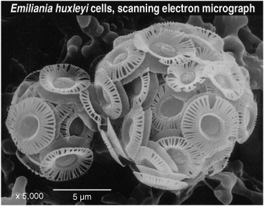
While the Dutch group set about trying to isolate the ketone-like compounds and decipher their structures, Sargent, who had always been concerned with the biochemical systems and ecology of live animals and had never given a lot of thought to their remains on the seafloor, was now ruminating about sediments and petroleum. He says Aberdeen was then in its boomtown days, and everyone was thinking and talking about oil, which somehow brought to mind an amusing lecture he’d heard at a Marine Biological Association meeting in Plymouth several years earlier, in 1971. It was about coccolithophores, a group of unicellular algae that were then known more for the tiny calcium carbonate shells they left as testament in marine sediments than for their living presence in the water. The shells of the most common species of the group, Emiliania huxleyi, comprised the bulk of many marine sediments and carbonate rocks, and were quite beautiful when viewed through an electron microscope. According to the speaker that day, “Emily,” as the Plymouth biologists fondly called the algae, contained a large oil globule that made it float near the surface of the water. The speaker innocently speculated that this oil might also accumulate in sediments and even have something to do with the formation of petroleum, and a rather rancorous but humorous argument erupted about how an oil that made coccolithophores float could sink into the sediments. So now Sargent found himself wondering if the unknown lipids he’d found in such quantity in the North Sea sediments might come from this same oil. Just for fun, he wrote to Plymouth and requested a starting culture of Emily.
The algae grown from the Plymouth culture, as it turned out, produced the exact same long-chain ketones his group had isolated from the North Sea sediment extract—an amazingly fortuitous result, given the string of free association that inspired him to request the culture. Their precise chemical structures remained a mystery, but they were clearly the same compounds, and so plentiful that Sargent figured they must be concentrated in some sort of droplet inside the cell, perhaps even the oil globules he’d heard described at the Marine Biological Association meeting. He would have liked to know more about the compounds and their biochemical or physiological roles, but he could find no reference to such oil globules in the literature and he was feeling pressured to get on with the work that his laboratory had been funded for. With no intention of publishing the results from the study, they stashed the sediment and algal extracts in the deep freeze and went back to work on their live zooplankton—until some six months later, when biochemist John Sargent happened to meet organic geochemist Geoff Eglinton.
In the fall of 1976, the DSDP ship made a port call in Aberdeen, and Geoff, as a British participant in DSDP advisory committees, was invited to tour the ship and join the reception and press conference, which was held at Aberdeen’s Institute of Marine Biochemistry, where Sargent worked. Sargent had nothing to do with the DSDP, but he wandered over to the reception just to see what was going on and get some free coffee. The two got to talking, and Sargent told Geoff about his foray into the sediments and the strange algal lipids he’d isolated. Geoff was immediately intrigued, and of course, when he heard that the Scottish team hadn’t figured out the chemical structures, the challenge was more than he could resist. “We can crack it!” he exclaimed enthusiastically, if a bit too optimistically. He headed back to Bristol with several vials of the mystery compounds from Emily, but then they languished in the freezer there for another year before anyone in the lab had the time, and the interest and particular skills, to analyze them.
Australian John Volkman came to the Bristol lab on a postdoctoral fellowship that was part of Geoff’s and James Maxwell’s plan to end the lab’s reliance on chance discoveries. They wanted to embark on a more concerted, tailor-designed investigation of lipids in marine plankton and bacteria. Volkman was fresh out of grad school, but he had already demonstrated a talent for instrumentation and an interest in marine natural products. Almost immediately upon his arrival from Australia, Geoff sent him off to Switzerland to learn the most cutting-edge techniques in capillary gas chromatography from the royal family of GC, the Grob family—a father-mother-son team of world-class analytical chemists. When Volkman started trying to analyze the Emily extracts and, like the Aberdeen biochemist, couldn’t get the long-chain ketones through the lab’s commercial GC columns, he was well prepared to make his own capillary columns. He used a material that could withstand the high temperatures needed to vaporize the unwieldy compounds, but they still got stuck in the injection system and he finally resorted to dipping the end of the column directly into his extracts. The reward was a chromatogram with eight clearly separated peaks, four from each band scraped off the thin-layer separation plates.
While Volkman was trying to figure out the structures of the Emily ketones, other Bristol postdocs and students were busy working on new DSDP cores from the Japan Trench, a deep ravine in the ocean floor immediately southeast of Japan. They were analyzing organic-matter–rich sediments that had been deposited during a period of high productivity, extracting, separating, and identifying as many of the lipids as they could. Simon Brassell, who was still a student at the time, was responsible for the steroid and ketone fractions. Using a standard, commercially available GC column, he was finding ketones that seemed to mirror the n-alkanes in chain length and distribution, and he suspected they’d been produced by bacterial oxidation of the alkanes in the top layers of sediment shortly after deposition. One day he forgot to turn the chart recorder off and by the time he remembered, paper was spilling out across the room. As he gathered it up, he noticed a massive, ill-defined hump as if something had bled off the column at the end of the chromatogram, long after the column had reached its maximum temperature and his ketones and everything else had come through. At first he was afraid that the material inside the column was breaking down, but a blank run produced only the expected long, straight line of nothingness. He purposely left his next sample running for an extended period, and the hump showed up again, now followed by several others. At that point, he decided to try running his Japan Trench extract on John Volkman’s new system and, lo and behold, the humps were replaced by 10 clearly separated peaks, eight of which matched those of Volkman’s Emily ketones.
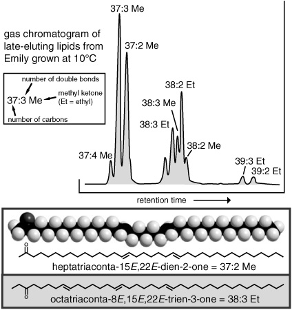
By this time, Volkman had identified eight different long-chain ketones, or “alkenones” as they came to be known, all variations on a theme: long unbranched carbon chains with several double bonds and a carbonyl group near the end, just as Sargent had deduced. They had from 37 to 39 carbon atoms and two or three double bonds, and the carbonyl was either at the C-2 position or the C-3 position. He was still trying to determine exactly where in the carbon chains the double bonds were positioned when Jan de Leeuw visited Bristol for a thesis defense. De Leeuw had a reputation for being a whiz at mass spectra interpretation, so Volkman showed him the alkenone mass spectra, in the hope that de Leeuw might be able to figure them out. To Volkman’s surprise, de Leeuw didn’t have to figure out anything—he recognized the spectra immediately and drew out the compounds, double bonds and all. It was the same compound his student Jaap Boon had found in a DSDP core from the Walvis Ridge. “What sediment is this from?” he asked Volkman, and then it was de Leeuw’s turn to be surprised: Volkman told him the compounds hadn’t come from a sediment but, rather, from an extract of the common marine coccolithophore Emiliania huxleyi.
With the realization that they’d been investigating the same compounds, the Dutch and Bristol groups began to swap information and samples. At the next international meeting of organic geochemists in the fall of 1979, they presented their papers together, detailing the structures of the alkenones and reporting their presence in a variety of marine sediments and in the coccolithophore Emiliania huxleyi. Volkman had followed Sargent’s lead and collaborated with the biologists in Plymouth, requesting cultures of a number of other algae and bacteria, but he found no alkenones in any of them, not even in other species of coccolithophores. He also analyzed some of the original milky water from the North Sea lemonade bottle, about which there was still some confusion, due to yet another coincidence that Sargent was initially unaware of: Emiliania huxleyi is often associated with just such a milky water phenomenon. When nutrients are high and their numbers swell, the billions of microscopic calcium carbonate shells make the water look as if it’s full of powdered chalk and create spectacular expanses of ghostly pale, turquoise-colored water that seafarers have been commenting on for centuries. It would have seemed quite logical for Sargent’s Emily quest to have begun with finding the ketones in the milky water the fishermen brought back, and in fact this is the myth that was and is still recounted in Bristol and beyond—that discovery of the alkenones began with a coccolithophore bloom in the North Sea. But the truth of the matter is that the water in the lemonade bottle was completely devoid of ketones and chock-full of copepod wax esters, as Volkman’s analyses confirmed. Sargent’s quest was more whimsical than logical. When he saw the alkenone structures he was curious anew about the biochemistry of the compounds—how they were synthesized and used, and if they were in fact concentrated in oil globules as he suspected. But he was too busy with his zooplankton to follow up, and the project was left to the geochemists … who had started finding alkenones in many of their DSDP cores, and noticing some very intriguing patterns.
Alkenones in Emiliania huxleyi
Simon Brassell had been working with DSDP sediments from the moment he’d started as Geoff’s research student three years before. For his doctoral thesis he had tracked the early stages of the complex web of reactions that converted the sterols in organisms to the steranes in petroleum and mature rocks that Andrew Mackenzie was working on with Maxwell. When he first noted that the distribution of the various alkenones in the Japan Trench sediments differed from what Volkman had found in his Emily cultures, he thought it was due to similar diagenetic reactions in the sediments. The algae contained mostly alkenones with three double bonds, whereas the sediments had a higher proportion of those with only two, so it seemed that the double bonds were gradually being reduced, just as the double bonds in sterols were reduced in the upper few centimeters of the sediments. Of course, there was also the possibility that some other, yet unidentified species made the same compounds in slightly different proportions. Other species must have made alkenones in the past, because he found them in segments of sediment core that were several millions of years old and, according to the fossil record of coccoliths, Emily hadn’t appeared on the scene until about 250,000 years ago.
While Brassell was working on the Japan Trench sediments, Geoff attended his first meeting as a member of the DSDP scientific advisory committee on paleoenvironments, a weeklong brainstorming retreat with a group of some fifteen oceanographers, geologists, and paleontologists. They were supposed to define the most pressing questions about conditions on Earth over the past 300 million years and recommend drilling sites in the world’s oceans, but the meeting was as memorable for its parasitic worms and nocturnal mosquito fests as it was for any daytime brainstorming. The meeting place was chosen such that all the international participants would have the shortest number of miles to travel, which somehow put them in a rather rustic, so-called conference center in Barbados. Geoff spent the hot, sleepless nights in conversation with the Austrian geologist he’d been assigned to room with: Michael Sarnthein, from the University of Kiel, heard about organic chemistry and molecular fossils, while Geoff learned all about the ice ages that geologists had spent the past century trying to understand.
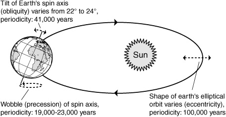
Naturalists had recognized signs of long-extinct glaciers and extremely cold climates in now temperate regions of the northern hemisphere at the beginning of the nineteenth century, but their attempts to explain the phenomenon all failed to account for later observations that there had been not one period, but multiple periods of glaciation that had alternated with periods of warmer climate over the past few million years. The most plausible explanation for such oscillations between glacial and interglacial climates was presented in 1930 by the Serbian mathematician Milutin Milankovitch, who suggested that it might be due to cyclical changes in the earth’s spatial orientation with respect to the sun. Milankovitch had determined that the slowly oscillating shape of the earth’s elliptical orbit around the sun, the shifting tilt of its axis of spin relative to the plane of its orbit, and the wobble in its spin would affect the distribution of solar radiation and intensity of seasons in cycles of 100,000, 41,000, and 23,000 years, respectively. The variations in solar radiation were minuscule, but he reasoned that they might be enough to trigger feedback effects. If, for example, the amount of sunlight decreased just enough that some patches of snow survived the summer, then the snowfields would build up over the years, reflecting away more sunlight as they expanded and amplifying the small cooling from the orbital changes, until the snowfield had grown, over the centuries, into a thick sheet of ice that covered half a continent. Based on these variations, Milankovitch estimated the climate fluctuations over the past 450,000 years and came up with cycles of cold and warm periods, the so-called Milankovitch cycles.
Orbital variations
Geologists were unable to determine the timing of the glacial periods from the rocks, and Milankovitch’s astronomic theory was just the hypothetical musing of a star-gazing mathematician until the 1970s, when the DSDP made marine sediments from around the world available for study in overlapping sequences of tens of millions of years, and chemists and paleontologists developed reliable means for dating them and estimating paleotemperatures. Paleontologists had spent nearly a century classifying the tiny fossils of unicellular zooplankton—the silica shells of radiolaria, and the calcium carbonate shells of foraminifera—and could distinguish tens of thousands of extant and extinct species. As they learned which species thrived where and at what temperatures, they developed statistical treatments of the relative abundances of microfossils that not only allowed them to correlate layers of sediments deposited during the same time period in different regions, but also provided some indication of the climate at the time. These techniques became increasingly difficult when the sediments were dominated by extinct fossil species, and were not very dependable for sediments that were more than 30,000 years old. Chemists soon learned, however, that the calcium carbonate shells of the foraminifera had an index of seawater temperatures built into the atoms of the mineral itself, and this was less dependent on the precise identification of species. When the shells precipitate from the dissolved carbonate in seawater, they preferentially incorporate carbonate that contains oxygen-18, the rare heavy isotope of oxygen, which has an extra two neutrons in its nucleus compared to oxygen-16. The lower the temperature, the stronger this preference for 18O: when researchers carefully picked out the tiny, millimeter-sized foram shells from the rest of the sediment and measured the relative amounts of 18O and 16O—a difficult undertaking in the 1950s, but an elementary task for a mass spectrometer in the 1970s—they could, theoretically, determine the temperature of the sea at the time the shells had formed.
The story that began to emerge from such painstaking analyses of marine sediment cores in the late 1950s was of a climate that had shifted back and forth between cold glacial and warmer interglacial periods dozens of times during the past few million years. And by the mid-1970s, Milankovitch’s theory had descended from the stars and settled, with dramatic certainty, in the solid realm of geologic evidence: researchers were able to combine 18O and microfossil species distribution data for DSDP cores spanning the past 450,000 years and, using established mathematical methods to determine their cyclical components, show that the cooling and warming periods alternated with frequencies that combined components of Milankovitch’s three orbital cycles.
Sarnthein explained to Geoff how he and others had been gathering data from DSDP cores in an attempt to both verify and understand these results. Though it was clear that the orbital cycles were in some way responsible for triggering the glacial–interglacial climate shifts, it wasn’t at all clear how. As Milankovitch himself had noted, such minuscule changes in solar radiation would have to set in motion other processes that magnified their effect. But it wasn’t clear what the timing of ice formation had been with respect to other climate variables. Indeed, there wasn’t even a clear picture of how the whole climate system had operated during the last ice age—what the wind patterns had been, the differences between land and ocean temperatures, patterns of heat-transporting ocean currents and deep ocean circulation.… Even the overall latitudinal temperature differential was unknown. First and foremost, they needed maps of sea surface temperatures dating back a few million years. Sarnthein said he and others had been trying to obtain enough microfossil species distribution and 18O data to construct such maps, but both techniques were incredibly labor intensive. Plus, in some areas of the ocean the calcium carbonate shells had dissolved before they reached the seafloor, so there were few fossils to be found and the technique was rendered completely useless. Another big problem, he said, was that the 18O to 16O ratios in fossil foram shells depended not only on temperature, but also on the 18O to 16O ratio in the ocean water, and this had not been constant. Evaporation and cloud formation preferentially removed H2O with the lighter 16O isotope; if rain and river runoff didn’t return all the evaporated water to the ocean, the water would become enriched in 18O, and this was what happened during an ice age when most of the rain that fell over landmasses was tied up in glaciers. The oxygen isotope ratios in the fossil forams thus gave an ambiguous measure of ocean temperature and ice volume.
What Geoff learned from Sarnthein during that Barbados “retreat” in 1979 was that oceanographers, paleontologists, and geologists—everyone who wanted to know anything about the climates, oceans, and ecology of the past, and even those who were trying to predict the future—were all desperate for an independent sea surface paleothermometer to fill in the gaps and clarify the intriguing but ambiguous message they were getting from the 18O data. A few months later, when Brassell came bursting into his office suggesting that the alkenone distributions in the sediments he’d been analyzing might be the result not of diagenesis but of the different temperatures in the water where the algae had been growing, Geoff realized that just such a paleothermometer might already be under design in his own laboratory. The oceanographers would call it a temperature “proxy” because it was a way to determine temperatures through a third party, so to speak, by measuring some other variable that acted in response to temperature. He looked at the chart of alkenone distributions Brassell showed him with a mix of jubilation and scientific cynicism—it was such a fantastic possibility, he thought, that it couldn’t possibly be true … or could it?
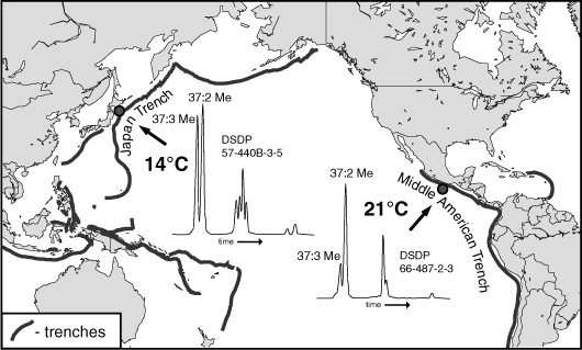
Brassell had been doing a preliminary write-up of analyses of a DSDP core from a site near the Middle America Trench, off the Pacific coast of southern Mexico, comparing the lipid distributions to those in his Japan Trench sediments from the same period, which extended from the present back to about five million years ago. Having finished his thesis on the diagenesis of sterols, he was on the lookout for anything that might link the various lipids the Bristol team was finding not only to their source organisms, but also to specific environments or processes. He noticed that the distribution of alkenones in the Middle America Trench sediments was, like that in his Japan Trench sediments, inconsistent with the distribution in John Volkman’s Emily cultures. But the cumulative alkenone data from all the cores the group had analyzed revealed none of the gradual, systematic changes with age that one would expect if the difference was due to diagenetic alteration. When he noted that the alkenone distributions in the Middle America Trench and Japan Trench sediments of the same age also differed dra-matically—that at the tropical site alkenones with two double bonds were much more plentiful than those with three double bonds, whereas in the Japan Trench sediments they were only slightly more plentiful—the most dramatic difference in the two environments came immediately to mind: in the modern ocean, at least, there’s a cold current running from the polar region south along the coast of Japan, whereas the water off the coast of southern Mexico is as warm as a baby’s bath.
Alkenone distributions: Japan Trench and Middle American Trench
Was it possible that the algae adapted to water temperature by changing the degree of unsaturation in their alkenones, making more double bonds if they lived in cold water, fewer if they lived in warm? For his part, Volkman says this possibility simply didn’t occur to him, despite having recently collaborated on a project where certain bacteria were found to vary the degree of unsaturation in their fatty acids as a means of maintaining the consistency of their cell membranes at different temperatures. He’d been working with biochemists at the time, not thinking about paleoenvironments or biomarkers. And when he did start thinking about them, the fatty acids were not in the running. Their carboxylic acid groups, relatively short carbon chains, and closely spaced double bonds made them too reactive and easily transformed; they were synthesized by all types of organisms, including bacteria in the sediments, and the species-specific distributions of chain length and unsaturation that could help to distinguish organisms were quickly lost during diagenesis in the sediments. But the alkenones were another matter altogether. They showed every promise of being perfect biomarkers: their excessively long carbon chains made them insoluble in water, immobile in the sediments, and presumably difficult to degrade; their double bonds were spaced far apart and relatively unreactive; they were unusual, apparently limited to a few species of algae; and Emiliania huxleyi, their main producer in modern times, was plentiful and cosmopolitan, present in all the world’s oceans except the Southern Ocean around Antarctica. That such a perfect biomarker might preserve a record of sea surface temperature seemed too good to be true … and so Geoff and Simon Brassell immediately sat down and listed all the reasons it might not work. Then they wrote a proposal to fund a graduate student project so it could be tested—outlining all the key experiments, but carefully avoiding direct reference to the suspected temperature dependence of the alkenones, just in case. They didn’t want to set some reviewer off on the same path and risk being scooped.
The first thing, of course, was to see if Emily really did manufacture different combinations of alkenones when grown at different temperatures, or if the differences observed in the sediments were the result of something else entirely. And then, too, were the alkenones really as sturdy and resistant to microbial attack as they looked? What happened to them before they got to the sediments? How did they even get there? Emily’s cells were so small that they were hardly visible under a traditional light microscope, just a thousandth the size of the copepods and foraminifera that fed on them. Calculations indicated that if the dead cells were left floating in the water column, it would take them more than a hundred years to sink the thousands of meters to the seafloor. Most phytoplankton, however, were eaten by zooplankton, whose millimeter-sized fecal pellets could sink in a matter of days and made up much of the organic component of the sediments. But wouldn’t a voyage through a zooplankton intestine have some effect on the structures of the alkenones?
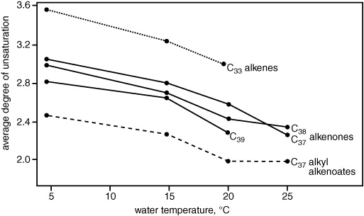
The Plymouth marine biologists and biochemists had been studying the fecal pellets of Emily’s most likely grazer, the copepod, for years, and Geoff sent Fred Prahl, one of the Bristol postdocs, to work with them. Together, they grew cultures of Emily, fed them to copepods, collected the fecal pellets, and extracted and analyzed the lipids—and found that the alkenones did indeed pass undigested and unchanged through the zooplankton intestines. The Plymouth group also started growing some cultures of Emily at different temperatures, and Ian Marlowe, the student funded by the paleothermometer proposal, was charged with analyzing their lipids. His first graph of temperature versus the ratio of diunsaturated to triunsaturated alkenones only had three points—at 20°, 15°, and 5°C—but it was enough to show a distinct trend toward more triunsaturated compounds with decreasing temperature. In addition to a series of related 37- to 39-carbon esters and simple alkenes that showed similar trends, Marlowe identified alkenones with four double bonds in the low-temperature cultures, and it became clear that the overall degree of unsaturation in the algae’s lipids increased systematically with decreasing temperature.
The Bristol researchers moved into high gear. They continued the collaboration in Plymouth, searching for alkenones in other species of algae and exploring factors other than temperature that might influence the distributions—the growth phase of the algae, the nutrient levels in the water, microbial activity, or chemical breakdown in the sediments. They searched for a single index that would reflect the temperature dependence of the overall degree of unsaturation in the family of long-chain compounds, and finally focused on the 37-carbon alkenones, which were the most plentiful and consistently present, and included only methyl ketones. They went on a massive data-gathering campaign that would eventually allow them to calibrate their unsaturation index against actual water temperatures, using the alkenone distributions not only in laboratory-grown cultures of algae, but also in natural populations of phytoplankton and marine sediments. And, finally, Geoff cut to the chase and contacted Michael Sarnthein.
Average degree of unsaturation versus algal growth temperature for long-chain unsaturated lipids in Emiliania huxleyi, 1982
Where could they obtain a sediment core to test their developing temperature proxy against the 18O record of the ice ages, he asked Sarnthein—one that spanned the last million years of glacial–interglacial climate cycles, had an uninterrupted record of forams for 18O analyses, and contained sufficient quantities of alkenones for their measurements? Sarnthein immediately recommended a site in the Kane Gap, off the coast of northwest Africa, where the German research vessel Meteor was scheduled to go in 1983. The Meteor wasn’t a big drill ship like the DSDP’s, but it could retrieve short gravity cores of 10 or 15 meters, which should serve their purposes, and Sarnthein already had a place secured as a principal researcher. He could easily take Marlowe along to collect the samples for organic analysis.
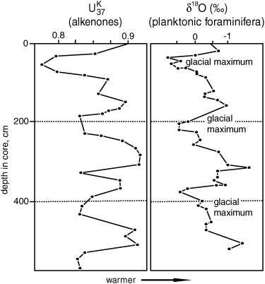
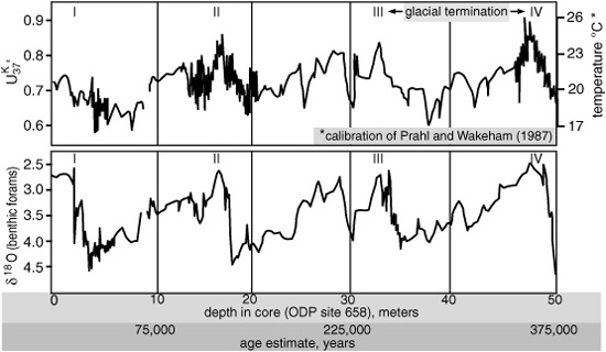
In the fall of 1984, four years after Brassell burst into Geoff’s office with his too-good-to-be-true proposition, members of the Bristol group met in London with Sarnthein to exchange and discuss their Kane Gap results. Geoff says he couldn’t make heads or tails of their alkenone data. They had plotted their unsaturation index based on the C37 compounds against depth in the core, but it just looked like a bunch of irregular squiggles. He apologized for its inelegance as he handed it to Sarnthein, but Sarnthein took one look at the graph and exclaimed, “That’s it! There they are! But it’s easier to follow if you flip it over.” Stable isotope compositions were usually given as “delta” values, he explained. δ18O was the amount that the proportion of 18O in a sample deviated from that in an ocean water standard and became more negative with increasing temperature, so he was accustomed to looking at what amounted to inverted temperature curves. He turned the Bristol group’s unsaturation index graph around and proceeded to explicate each of the little squiggles in terms of the waxing and waning glaciers that he and others had been seeing in the δ18O data from sediment cores around the world.
Alkenone unsaturation  and oxygen isotope (δ18O) stratigraphy Kane Gap core, east equatorial Atlantic Ocean, 1984
In Bristol they were still working to calibrate their unsaturation index with seawater temperature, so they couldn’t put precise sea surface temperatures on their graph. In the months that followed the meeting with Sarnthein, they finally settled on the unsaturation index that gave the best calibration, would increase with temperature and give values that conveniently varied between 0 and 1. They named it  for unsaturation, K for ketone (with a nod to national vanity), and 37 because they’d limited it to the 37-carbon compounds—and defined it as:
 = (C37:2 – C37:4) / (C37:2 + C37:3 + C37:4),
where C37:2 was the concentration of compounds with 37 carbons and 2 double bonds, and so forth. When Geoff displayed Sarnthein’s δ18O data, plotted right-side up, along with plotted upside down, at the next international organic geochemistry meeting, the excitement in the room was palpable: the ice-age climate oscillations were as apparent in the biomarker data as they were in the foram data, which, of course, were registering the combined effects of changing temperatures and changing ice volume. It was the 12th International Meeting on Organic Geochemistry, held in Jülich in the fall of 1985, and it was packed: what had been a scattered handful of maverick chemists and geologists when Geoff extracted his first hunk of Green River shale two and a half decades before was now a community of organic geochemists some 400 members strong. Purely by chance, Geoff had been scheduled to present the first paper of the conference, and for the rest of the week people would stop him in the hall to remark on the Bristol-Kiel cooperative and offer congratulations and encouragement: the alkenones had set the community abuzz. There was a sense that organic geochemistry had crossed a new threshold and was ready to take on some of the most interesting and difficult questions in the earth sciences.
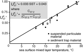
Complete results from the study appeared in a 1986 paper in Nature under the audacious title “Molecular Stratigraphy: A New Tool for Climatic Assessment.” As intended, the paper captured the attention of the oceanographic community, including the once-disdainful marine geologists and paleoceanographers. For their part, the marine chemists at Woods Hole had been interested in the alkenones since John Volkman had visited them in 1980, well before anyone had any idea that they might be useful as a paleothermometer. Max Blumer had died in 1977, but his legacy of marine organic chemistry at Woods Hole lived on in the work of John Farrington, Bob Gagosian, and Cindy Lee, who had been analyzing everything from hydrocarbons and sterols to the cycling of amino acids in the water. When Volkman visited, Stu Wakeham had recently joined their ranks and was developing new and improved methods of collecting suspended and sinking detritus from different depths. The group immediately added the alkenones to its repertoire and found it to be the most stable of the compounds made by marine organisms that they had come across. Not long after the paleothermometer was unveiled, Fred Prahl, who had worked on the coccolithophore feeding experiments in Plymouth, also did a stint at Woods Hole, teaming up with Wakeham to determine values from the alkenones in sinking and suspended particles. Plotting these against temperatures in the overlying surface water from a range of environments produced a surprisingly straight line that was remarkably close to the one determined from the alkenones of Emily grown at different temperatures in the laboratory. This served to calibrate the new paleothermometer, though efforts to extend, refine, and validate that calibration would continue for another decade.
Geoff had started the Bristol group collecting data for a definitive calibration of as soon as he’d seen Marlowe’s first graphs. But he’d reasoned that such a calibration should be based on a broad survey of marine sediments—where seasonal temperature changes, biological effects, and diagenetic loss of the alkenones would all be empirically averaged out—and it took years to acquire the requisite surface sediment samples from all the world’s oceans. In the meantime, the group tried to determine if any extant organisms other than Emiliania huxleyi made alkenones, and what the source of the compounds in the sediments might have been before Emily came on the scene. Marlowe did a study of cores that extended back into the middle of the Eocene epoch to about 45 million years ago, comparing alkenone distributions with the microfossil records in the same sediments. Paul Farrimond, another student of Geoff’s who was working on a completely different project, forgot to turn the chart recorder off after a GC run and discovered quite by accident that alkenones were present in the 100-million-year-old Cretaceous sediments he was analyzing. The hunt for alkenones in living algae eventually revealed their presence in a handful of closely related species, all, like the coccolithophores, members of the Haptophyta division, and, with the exception of Emily, uncommon in contemporary oceans, or limited to coastal regions. Later, in the mid-1990s, Volkman and his colleagues in Australia would find alkenones in Gephyrocapsa oceanica, which can be as plentiful as Emily in tropical or marginal seas. This may well have been a main source of alkenones in the past, as Gephyrocapsa coccoliths comprise the dominant form of haptophyte fossil for the three million years or so before Emily took over the show.
Calibration of  from suspended and sinking particulate matter, 1987
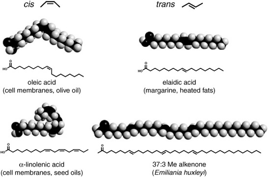
Volkman says there was a period after he left Bristol when he just couldn’t get away from the alkenones, even when it seemed most unlikely he would encounter them. By the mid-1980s, he was back in Australia with a post at the Marine Research Division of the Commonwealth Scientific and Industrial Organization, and he and one of his students were studying the ecology and history of a large saline lake in Antarctica, analyzing lipids and pigments in its sediments. The Southern Ocean is one of the few regions of the world where Emily doesn’t live, so though the lake was quite saline and had been connected to the sea in the past, they were surprised to discover that the sediments deposited at various times in its history were loaded with alkenones—so loaded, Volkman says, that he and his student were able to obtain their infrared spectra. The compounds with four double bonds predominated, as might be expected in such a cold region, but the species responsible couldn’t be identified, and when they tried to get a record of the lake’s temperature from the proxy, it gave unrealistic values—highlighting the necessity of defining limits to the proxy’s use in areas and periods of time when Emily was not the main alkenone producer. More importantly, the infrared spectra revealed a hitherto unnoted quirk in alkenone molecular structures, which had, to date, still not been confirmed by synthesis: of the two geometric forms possible for double bonds, cis and trans, the alkenone double bonds seemed to be trans, a very unusual configuration for straight-chain biological lipids and confined to a few special cases, such as in carotenoid pigments. Maxwell had a post-doc in Bristol trying to synthesize the cis alkenones in the laboratory, so Volkman immediately sent him a note. Sure enough, when they changed tactics and accomplished the difficult syntheses, they duplicated the compounds made by algae and found in the sediments, replete with all-trans double bonds—but how the algae themselves accomplish this synthesis remains a mystery to this day.
cis and trans double bonds in fatty acids and alkenones
Until very recently, it wasn’t even clear where in the cell the alkenones reside. The Bristol group speculated that they were bound in the cell membrane, and that the change in saturation was a means of regulating its viscosity or fluidity at a wide range of temperatures, as had been observed for fatty acids in some bacterial membranes. This speculation has been repeated as if it were documented fact in just about every alkenone paleothermometer reference since 1986, but there were, in fact, few investigations into its verity. Sargent and Maxwell had wanted to set up a graduate student project to study the biochemistry of the alkenones, but there just wasn’t funding for such basic research in the 1980s and 1990s. For his part, Sargent says he never subscribed to the idea that the alkenones were membrane-bound lipids. His Scottish brogue makes everything sound like a question, but there’s nothing questioning in his opinion on the subject. “That’s just rubbish,” he says bluntly.
Sargent claims the alkenones are too long to fit into the membrane, for one thing. And whereas cis double bonds in fatty acids give them a kink that fits loosely into the flexible membrane, the trans double bonds make the molecule into a straight, rodlike structure that seems an unlikely choice for a membrane lipid. Furthermore, Sargent says, there is no way that the large amounts of alkenones found in Emily cells could be bound to the cell membrane. There must be globs of them inside the cell, enclosed in little vesicles of some sort—quite possibly the same oil globules he’d heard described by the Marine Biological Association biologist back in 1971. Indeed. Not long after I talked to Sargent in 2004, more than two decades after the discovery of the alkenones, biochemists began making concerted attempts to ascertain their position in the cell and found that they are not, in fact, bound in the cell membrane as most of the geochemists had been assuming. Just as Sargent expected, the entire series of alkenones and related compounds appears to be contained in vesicles of oil inside the cell, and there is now significant evidence that they are used for energy storage much like more conventional fat molecules are used in other algae. But why, then, is the degree of unsaturation temperature dependent? We seem to have returned to first base with this question.
Certainly understanding the biochemistry of the alkenones would help in their use as a paleotemperature proxy, which is ultimately dependent on the consistency of that biochemistry during the evolution and diversification of alkenone-producing species. The sources of the alkenones found in sediments that predate Emily’s emergence remain a matter of speculation, and laboratory culture studies with the handful of extant alkenone-producing species indicate that the temperature dependence of alkenone unsaturation can vary significantly among species, and even between strains of algae obtained from two different geographical regions. There are also concerns that the temperature dependence might be nonlinear at lower temperatures or that triunsaturated alkenones degrade more quickly than diunsaturated.… And confusion reigns about whether the alkenone signal represents average annual temperatures, or is skewed toward spring and summer when the algae are at their peak, or whether, on the contrary, it is biased toward the low-nutrient periods in the surface water when the algae produce more alkenones to store energy they can’t use.… But amid all these ifs, buts, and maybes—and now, without even a working hypothesis to explain the correlation between water temperature and the degree of unsaturation to begin with—compilations of average annual sea surface temperatures and values from surface sediments around the world yield a consistently linear relationship, and after years of challenges and recalibrations, the equation that is still used to assign average annual sea surface temperatures to measurements of in ancient sediments is almost identical to the one first derived from sediment trap data at Woods Hole in 1987. And not long after its introduction, it started to yield new—and surprising—information about past climates, information that has played a part in a virtual paradigm shift in ideas about how the earth’s climate system operates.
By the end of the 1980s, the idea that climate change during the past hundred million years was driven primarily by plate tectonics and the earth’s orbital geometry had become a paradigm, supported by a large body of evidence from ocean sediments. The picture that had emerged was of a climate system that changed very gradually, over millions of years, in response to factors associated with the slow movement of the earth’s tectonic plates and concomitant uplift, subsidence, and volcanism—shifting continents, changing topography and ocean currents, and changing concentrations of atmospheric CO2. The earth’s orbital cycles caused average global temperatures to oscillate, with frequencies of 40,000 and 100,000 years, around the mean determined by this gradually changing climate system, which over the past 60 million years had become progressively more sensitive, with the oscillations growing in amplitude.
Worldwide calibration of in surface sediments (1998)

Abundant geologic evidence indicated that as long as the earth was free of ice, as it appears to have been throughout the long Cretaceous period and perhaps even back to the beginning of the Mesozoic era some 248 million years ago, the climate’s response to orbital variations was limited. But when ice began to form in Antarctica about 33 million years ago, after a prolonged period of gradual cooling in the Eocene, subtle 40,000-year oscillations in global climate began to appear in the geologic record, increasing in amplitude as the amount of ice increased. Presumably, conditions on Earth were now such that the small variations in the angle and intensity of incoming solar radiation were triggering the feedback effects imagined by Milankovitch: the tendency of the ice to reflect heat back into space, or alterations in ocean circulation due to the changing salinity and density of ocean surface waters as ice melted or formed. When ice began to form in the northern hemisphere a little more than three million years ago, the oscillations increased dramatically in amplitude, first at 40,000-year and later at 100,000-year intervals, and eventually gave way to the bimodal, glacial–interglacial cycles that have characterized the earth’s climate for the past million years.
Throughout the development and reign of human beings, according to this paradigm, the climate had alternated between long, steady periods of cold and warm, separated by transition periods where glacial ice advanced or retreated, sea levels fell or rose accordingly, and temperate sea surface temperatures decreased or increased by as much as 6°C over a relatively short, 10,000-year period. So went the most popular version of the story. But despite the clear association of the Pleistocene ice ages with the Milankovitch cycles, and despite evidence of feedback effects in the earth’s internal climate system that could have been triggered by small variations in the distribution and magnitude of solar heating, no one had come up with a plausible combination of feedbacks that produced large enough effects to account for the switch from ice age to interglacial period, or vice versa.
Most paleoclimate analyses required tediously picking through each sample to find well-preserved fossil shells, which were sometimes few and far between. And since some species of foraminifera were planktonic and some lived on the seafloor, the only way to distinguish the temperatures at the sea surface, which was in contact with the atmosphere, from the much colder and less variable deep sea temperatures was to pick out a chosen species one by one. Alkenone analyses, however, could be performed rapidly on small samples of bulk sediments. In coastal zones or other areas with lots of nutrients and high primary productivity in the surface waters, the sediments accumulated fast enough that one could obtain such samples at relatively short time intervals and, potentially, obtain a more detailed record of climate change during the Pleistocene than had to date been possible.
In 1991, scientists from the Bristol-Kiel alliance obtained just such a record from alkenone analyses of sediments in a core taken off the northwest coast of Africa, where they were able to sample at one- or two-centimeter intervals, about every 75–200 years, over part of the past 650,000 years. The last three ice age cycles were readily apparent in the data, with glacial to interglacial transitions beginning 340,000, 250,000, 150,000, and 25,000 years ago. But superimposed on this now-familiar climate curve were rapid fluctuations in sea surface temperature, sudden leaps and dips of several degrees that occurred within 300 to 1,000 years—fluctuations that clearly weren’t triggered by Milankovitch’s orbital cycles, and less so by tectonic factors. So surprising were the results, Geoff says, that when they submitted their paper to Nature, the reviewers objected, saying that temperature changes could not possibly be that fast, and when the paper did appear, duly fortified with more data, it was received with some skepticism. Hypothesis-loving geologists were loathe to sully their neatly oscillating oxygen isotope curves and eloquent, if incomplete, astronomical explanation with such baffling patterns of temperature swings—especially when they came from an unorthodox method.
First alkenone record of abrupt climate oscillations,1991: Comparison with the foram δ18O record during three glacial cycles (tropical NE Atlantic)
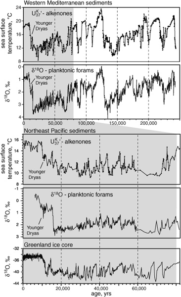
There had, in fact, been some scattered evidence of abrupt climate changes in the North Atlantic during the last glacial period, but it had hitherto been dismissed as a regional phenomenon. The alkenone evidence, however, came from a tropical region and indicated that the changes were global in nature … and fast on its heels came verification and clarification from other methods and cores. Analyses of the 18O content of ice samples from cores drilled deep into the ice sheets covering Antarctica and Greenland—ice that had accumulated in annual layers during tens of thousands of years—showed a similar pattern of rapid change. And as the Ocean Drilling Program (the DSDP’s successor in the 1980s and 1990s) retrieved more sediment cores where high-resolution studies were possible, further alkenone and improved 18O analyses of foram shells confirmed that abrupt climate oscillations had indeed affected the entire globe.
It was fast becoming clear that the long glacial and interglacial periods of the Milankovitch climate cycles were not as stable, and the transitions between them were not as decisive, as hypothesized. Rather, the earth’s climate had flickered back and forth between warm and cold modes every 2,000 years or so, with sea surface temperatures dropping some 4°C within a few hundred years, even in tropical regions. Joan Grimalt, who participated in the initial development of the index when he was a postdoc in Bristol, went on to refine its use and application in paleoceanographic studies of the Mediterranean and North Atlantic. One recent study by his Barcelona-based group shows that the climate flickers occurred throughout the past 250,000 years and that they were generally more frequent during glacial than during interglacial periods, and most pronounced during the transitions from interglacial to glacial. Indeed, after a relatively long period of interglacial stability like the current one, the temperature swings could be so dramatic as to flip the climate from interglacial to glacial and back again in the space of a few hundred years.
Records of abrupt climate oscillations: alkenones and δ18O
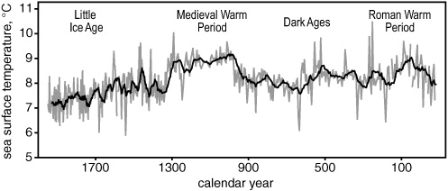
Still more detailed investigations of Holocene sediments, and more and better ice core measurements from Greenland, have brought the paleoclimate record into historical time, where the only abrupt climate change was much more subdued than those that punctuated the last three glacial cycles—but nevertheless wreaked havoc on the developing civilizations of Northern Europe. Around the turn of the fourteenth century, a 300-year period of mild weather and stability known as the Medieval Warm Period—a time when grapes were grown in England and the Vikings thrived in Greenland—ended abruptly, and the climate shifted gears. Within a few decades, Greenland’s coastal settlements were buried under its advancing ice cap, and the seas around Iceland were clogged with ice for months at a time, while the Thames River was freezing over in the winter. Dutch artists immortalized the era with romantic winter landscapes of ice-skaters frolicking on Amsterdam’s canals, but the four-century period known as the Little Ice Age was, in fact, a time of erratic weather, devastating storms, unpredictable crops, famine, epidemic disease, and die-out in Europe’s established population centers. As Grimalt points out, the climate shift in the fourteenth and fifteenth centuries was a minor blip compared to the abrupt changes in the global climate system that left their mark in the sediments of the world’s oceans during the last three glacial cycles. The most recent, known as the Younger Dryas, occurred about 11,000 years ago, as Earth was emerging from the last ice age, and flipped the global climate system back into glacial mode for another thousand years. And yet statistical analysis of the pacing of the Little Ice Age suggests a common external trigger for it and the earlier, more severe, abrupt changes.
From paleoclimates to historical climates: an alkenone  record of sea surface temperatures off the north coast of Iceland
This was a more precariously balanced climate system than anyone had suspected. As paleoceanographers began exposing and deciphering its record in the 1990s, the climate scientists who had been trying to model the physical and chemical processes that determine climate, making ever more complex calculations on ever larger computers to predict the effects of human additions of greenhouse gases to the atmosphere, started paying closer attention and using the long records of Pleistocene climate change to tune and calibrate the models. What tripped the switch and flipped the climate from one state to another so abruptly? What determined the extent and severity of the changes? Was it possible that man’s intemperate appetite for black gold—that burning hundreds of millions of years worth of Nature’s alchemy to CO2 in a couple of centuries—might trigger one of these sensitive features of the system and flip the climate suddenly into an unexpectedly extreme condition?
The climate scientists had found that when they increased the amount of atmospheric CO2 in their models, the initial warming in the Northern Hemisphere resulted in a complete reorganization or slowing of the deep sea circulation, which, in the contemporary ocean, functions like a giant conveyor belt, moving large amounts of heat from the tropics to high latitudes. This conveyor takes more than a thousand years to make its round and depends on the sinking of particularly dense water—cold and saline—at certain strategic points near the poles, its movement along the bottom of the deep ocean basins, and eventual upwelling and return flow in warmer, wind-driven surface currents.
Deep ocean circulation had long been considered one of the more stable features of climate, gradually readjusting itself over millions of years to fit the changing geography of the continents and topography of the seafloor. Theoretically, however, it could function in several distinctly different modes even within the constraints of the current geography and topography. If the water in those strategic locations near the poles changed in density, then the conveyor might slow or strengthen; if, for example, the water warmed or became less salty, the conveyor might shut down altogether, leading, ironically, to dramatic cooling in the North Atlantic and Europe. What had the climate scientists worried was that the new paleotemperature evidence from ice and sediment cores indicated that the great ocean conveyor had, in actuality, changed modes or pace, abruptly and repeatedly, in the past few hundred thousand years.
The precise cause and nature of these changes in deep sea circulation were unclear, but they appeared to be tied to the most dramatic of the abrupt climate flickers and to the glacial–interglacial cycles, part of a complex web of biological and chemical changes that were linked to the earth’s orbital cycles and, apparently, to the internal cycles of its moody sun, amplifying or modulating the effects of both. One of the most tangled and least understood strands of that web was one that geologists had generally failed to recognize until the 1970s: the productivity of microscopic algae living in the sunlit surface waters of the world’s oceans. In most regions of the open ocean, there is little mixing between the warm lens of surface water and the cold deep water, such that essential phytoplankton nutrients such as nitrate and phosphate become depleted at the surface, where all the photosynthetic action is, and enriched in the deep water where bacteria break down the sinking detritus and remineralize the organic matter. Nutrients are replenished to the surface waters by dust-bearing winds or river runoff from the continents, or by upwelling of the nutrient-rich deep water. The latter occurs along certain coastlines, where the winds create offshore surface currents that pull the deep water to the surface, and along the equator, where divergent surface currents have a similar effect. Changes in wind direction or intensity, changes in seasonal weather patterns, or changing sea level and the resultant shifts in continental runoff during the waxing and waning of the ice sheets—all would have affected availability of nutrients in the surface waters. Changes in the availability of nutrients meant changes in marine productivity which, according to the so-called “biological pump” hypothesis, might have amplified all these effects by generating fluctuations in atmospheric CO2 with associated warming or cooling as algae “pump” CO2 out of the surface waters and convert it to organic matter, some small fraction of which persists in deep waters or sinks to the seafloor and is buried.
Ocean circulation: the great conveyor belt
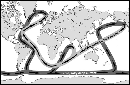
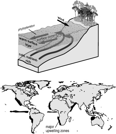
Paleoclimatologists and oceanographers have yet to decipher all the patterns of cause, effect, and feedback that comprise the earth’s climate history, but they have made headway in documenting some of its many components, either from analyses of the Greenland and Antarctic ice cores, where air bubbles trapped in the ice provide a record of the concentrations of CO2 and methane in the atmosphere, or from the longer mineral and fossil record preserved in a growing inventory of deep sea sediment cores. In the 1990s, they were joined in their endeavors by a new generation of organic geochemists: buoyed by the success of the alkenone paleothermometer and the growing realization that life was not a passive bystander, but a shaping force of the earth’s atmosphere, oceans, and rocks, the so-called “stamp collectors” were gaining a foothold in earth science and oceanographic institutions and were no longer relegated to the fringes of chemistry departments or constrained by the narrow interests of the petroleum industry. Jan de Leeuw moved his laboratory from Delft to the Netherlands Institute of Sea Research on the North Sea island of Texel, and “the Dutch group” became known as the NIOZ group. Jürgen joined the Institute of Chemistry and Biology of the Marine Environment at the University of Oldenburg; John Hayes, who was busy developing what would prove to be the most important new analytic technique for biomarker research since the GC-MS, created an official biogeochemistry group under the auspices of the geological sciences department at Indiana University; Geoff moved on to emeritus status at Bristol and joined the Woods Hole faculty as an adjunct scientist; and James Maxwell stayed put as Bristol’s guiding light amid a steady flow of students and postdocs from oceanography and earth science departments around the world. Decades of molecular exploration were beginning to pay off. Hundreds of molecular fossils had been identified in sediment extracts, some semblance of a lexicon for interpreting them had been developed, and one could begin to use them, along with paleontological and mineral-based information, to reveal new facets of earth history, including how marine productivity and ecosystems have changed over the past few million years of oscillating climates.
One of the keys to detecting and understanding changes in marine productivity lies, ironically, in being able to identify organic matter that came from the continents, and here, of course, Geoff’s old buddies the leaf wax n-alkanes play a major role. Darwin had noted in The Voyage of the Beagle that large amounts of wind-borne dust could be found far out to sea in the Atlantic Ocean, an observation that had always intrigued Geoff. By the early 1970s, when he started asking around about getting dust samples to analyze, oceanographers and geologists had already devoted quite a bit of effort to studying its movements and mineral properties, but they still couldn’t always pinpoint its origin. Wind-borne dust from desert areas was composed mostly of mineral matter, but it could also come from exposed soils and dried lake beds, which contained some component of highly oxidized organic matter, or from vegetated areas where the wind had picked up pollen and plant spores. The clay particles and trace metals in the dust provided some information about the source of the mineral matter and the patterns of the winds; likewise, the different types of plant pollen and spores might have something to say about the vegetation the winds had passed over. Geoff’s first question was, as usual: What sort of organic compounds are in there? Shouldn’t there be some molecular remnants of land plants, and then could they tell which land plants? Quite fortuitously, around this same time Al Burlingame sent him a student who had been working on the DSDP cores in Berkeley. Bernd Simoneit suspected that much of the organic matter he found in the marine sediments, even in the middle of the Atlantic, had actually come from the continents, and was curious about its provenance. He also happened to be married to an airline stewardess who could get him free tickets to all sorts of exotic places, so he was able to fly all over the world to set up dust-collecting stations and visit the odd handful of scientists who had assembled collections for one reason or another.
Not surprisingly, the long-chain n-alkanes, n-alcohols, and fatty acids from leaf waxes were among the most prominent organic constituents of this material, more prominent even than they were in river-borne sediments. Bob Gagosian and colleagues at Woods Hole studied collections of dust from the South Pacific, with a similar result, finding these leaf wax compounds in dust collected from an atoll more than 5,000 kilometers from the nearest land source. Apparently, the wax particles could be blown off the leaves by strong winds, or rubbed off by the abrasive mineral particles in the dust. But the organic matter that came from the soils and dried lake beds had already undergone extensive decomposition and oxidation—more so than that in sediments from rivers and runoff, which often contain whole pieces of decaying plant matter. When found in marine sediments, then, the refractory leaf wax hydrocarbons—in particular, the C29 and C31 n-alkanes and the C28 n-alkanol—can give a measure of how much organic matter has been transported from the continents to the ocean, either blown out to sea on the wind or deposited along continental margins by rivers. Simoneit’s analyses of the leaf wax hydrocarbons in dust, and the subsequent years of sediment analyses, also revealed recognizable geographical patterns in the chain-length distributions of these long-chain compounds that seemed to correlate with the sources of the dust. And, finally, in recent years it has emerged that the chain-length distributions of leaf wax hydrocarbons do systematically reflect plant type, though at a much more general level than Geoff had searched for in his initial studies of Canary Island succulents: plants adapted to relatively warm, dry environments make more of the longer chain compounds, and those adapted to cool, humid environments make more of the short-chain ones.
All the interesting and potentially informative triterpenoids that have been isolated from plants seem to be largely absent, or present in trace amounts in dust, presumably having succumbed to oxic degradation in the soils. But what about in the sediments deposited by rivers and runoff along the continental margins? This was something Jürgen wondered about for years. Of the many pentacyclic triterpenoid structures that had been isolated from higher plants, the only carbon skeleton that showed up regularly in ancient sediments and oils was oleanane, the reduced analogue of β-amyrin. Oleanane, in fact, was inexplicably abundant and widespread. Natural products chemists had isolated β-amyrin from the leaves of some flowering plants—but they had also isolated lupeol, friedelin, taraxerol, and a host of other pentacyclic triterpenoids. Why so much oleanane, then, and so few of the other carbon skeletons that one might expect? Jürgen started puzzling about this during his first years in Dietrich Welte’s lab in Jülich, but not until the late 1980s, when he started analyzing Ocean Drilling Program sediments from Baffin Bay, did he and his colleagues stumble on an answer. Here, finally, buried hundreds of meters below the surface in the thick layers of sediments deposited by rivers and runoff from Greenland and Canada, they found some of the missing land plant pentacyclic triterpenoids—along with a plethora of triterpenes and related aromatic compounds that showed every indication of having been produced by dehydration and reduction of the biological alcohols and ketones, much as had been observed for sterols. Jürgen was working with two postdocs at the time, Lo ten Haven from NIOZ and Torren Peakman from Bristol, and they were struggling to identify all the triterpenes in the gas chromatograms in time for the ODP deadline on postcruise reports when they ran the hydrocarbon fraction of one of their extracts through a molecular sieve to remove the n-alkanes, one of which was coeluting with the triterpenes. To everyone’s surprise, the sieve not only removed the n-alkanes, but changed the composition of the triterpenes: the compound they’d been trying to quantify, taraxerene, disappeared, and the amount of oleanene increased. A survey of the literature revealed laboratory experiments that showed how taraxerene and a number of other triterpenes were converted to oleanene in the presence of an acid catalyst—in this case, it seemed, the acidic zeolite of the molecular sieve. In a mechanism similar to the one that had been proposed for the rearrangement of sterenes to diasterenes, addition of a proton to the double bond generates a reactive charged intermediate wherein the double bond of the triterpene is able to migrate around the ring structure, with concurrent rearrangement of the attached methyl groups.
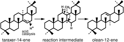
By the late 1980s, the Dutch had started doing theoretical molecular mechanics calculations to determine which of the sterenes produced by rearrangement of steroids were the most stable and energetically probable, and application of their findings to the triterpenes in the Baffin Bay sediments indicated that acid-catalyzed rearrangement of most of them would lead to one product: olean-12-ene. Careful quantitative analysis of the various triterpenes in the layers of sediment from the Baffin Bay core then revealed the answer to the oleanane riddle: in the relatively acidic clay-mineral–rich sediments generated by erosion of landmasses, triterpenes formed during the first stages of diagenesis converged on olean-12-ene, which further experiments indicated would slowly be reduced to the same mixture of oleanane isomers observed in more mature organic matter, only the most stable of which would survive in crude oils. It was a wonderfully eloquent bit of chemistry to discover in Nature’s messy sedimentary laboratory, and it reinforced what the Dutch had been seeing with their theoretical studies: in early diagenesis, when kerogen didn’t confound the issue, the reactions in the sediments could be predicted from first principles of chemical reactivity and thermodynamics.
Solving the oleanane riddle: proposed scheme for the diagenesis of pentacyclic triterpenoids from plants
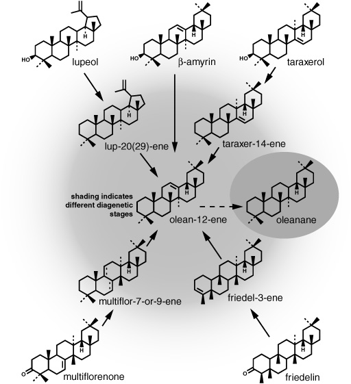
If, as appears to be the case, triterpenoids are largely absent from wind-borne dust, but present in river runoff, oleanene found in open ocean sediments can be used as an indicator that river-borne sediments from the continental shelf have been transported out to sea by bottom currents or submarine landslides. One even wonders if oleanene in coastal sediments might be used together with the n-alkanes to gauge changes in the relative input of organic matter from rivers and winds, or to detect a shift in the ecosystems on land, from triterpenoid-producing conifers, say, to grasses or deciduous forest. Another compound that is largely absent from dust and may be used to distinguish river-borne from both algal and wind-borne organic matter in marine sediments is lignin, the large polymer that provides structure and rigidity to land plants, most notably in the wood of trees. Unlike the steadfast n-alkanes, however, these compounds present serious problems with quantification and interpretation, as lignin breaks down into a dizzying array of difficult-to-analyze phenols, and the pentacyclic triterpenoids may well vary in their rate of survival during the sojourn from plant to river.
In an attempt to estimate past changes in marine primary productivity directly, the Bristol team returned to the roots of the biomarker concept and went straight to the heart of the matter: the green, light-absorbing chlorin heart of chlorophyll that Alfred Treibs had so cleverly linked to the red porphyrins in petroleum in the 1930s. Unlike phytol from chlorophyll’s tail, chlorins break down rapidly in the presence of light and oxygen, and on land they are destroyed in the dying leaves or soil, long before they can be transported to marine sediments. So the chlorins in marine sediments come only from the chlorophyll of marine organisms—algae or photosynthetic bacteria—unlike phytane, which could have come from land plants or even, for that matter, from the lipids of nonphotosynthetic microbes. Chlorins are also rapidly broken down in the marine environment, but some fraction persistently reaches the sediments and can be preserved for millions of years before being transformed to the refractory porphyrins found in ancient rocks and mature oils. The problem with trying to use chlorins as a measure of marine productivity in deep sea sediment cores from the Pleistocene—besides that they break down if samples are exposed to light or oxygen—is that they aren’t volatile enough to run on a GC-MS system. But in recent years Maxwell and his students have developed a method that uses high-performance liquid chromatography (HPLC)—a modern, automated version of the old column chromatography, where the stationary phase is a solid powder packed into a narrow steel column, the solvents are pumped through at high pressure, and both the rate and the mixture of solvents can be carefully controlled and gradually changed. Using such a system, chlorins are easy to separate from the mixture in a sediment extract and can be detected and quantified by an ultraviolet or fluorescence detector connected to the column outlet. The absolute concentrations of chlorins in marine sediments, then, can be used as an index of increases and decreases in marine primary productivity over the past few million years.
Specific information about which photosynthetic organisms are doing the producing and how the ecosystem changes over time comes from some of the many algal biomarkers that have been identified, often combined with paleon-tological inventories of the fossil shells and cysts. The amounts of alkenones can provide an index of coccolithophore activity, and dinosterol provides a relatively unambiguous record of dinoflagellate activity. Diatoms, which comprise almost half of the world’s total marine productivity in the contemporary ocean, are somewhat more difficult to pin down. Like coccolithophores and dinoflagellates, they form hard encasements that can persist as fossils in the sediments. But the delicate diatom frustules are made of silica, which is even more prone to disintegration than the calcium carbonate coccoliths or the organic dinoflagellate cysts, and their fossil record is even more patchy and undependable. Nor can they, to date, boast a “perfect” biomarker. Numerous sterols have been found in various groups of diatoms, but they all overlap to some extent with sterols made by plants and other algal classes: brassicasterol has also been found in coccolithophores, 24-methylenecholesterol—with its double bond between the 24- and the 28-carbon—has been found in some dinoflagellates, fucosterol in brown algae, β-sitosterol in higher plants. In Pleistocene marine sediments, where the sterols have yet to succumb to diagenesis, brassicasterol is often used as an indicator of diatom activity, but it appears to be made by only a few of the many diatom genera and, like all of these compounds, is best measured as part of an array of biomarkers. In older and more mature sediments where the sterols have been reduced to their sterane skeletons, only dinosterane with its distinctive 4-methyl group preserves its source-specific structure, but one can get a rough idea of the relative contributions of higher plants, marine algae, and zooplankton from the side-chain substitution patterns and relative amounts of 29-carbon, 28-carbon, and 27-carbon steranes, respectively. The carotenoid pigment fucoxanthin is particularly abundant in diatoms, and under some conditions its cyclic components are preserved in the relatively stable and distinctive loliolides, which can thus provide clues to periods when diatoms were particularly productive.
Another ambiguous but potentially useful biomarker for diatoms was identified by Jaap Sinninghe Damsté and the NIOZ group when they went on a natural products offensive and started growing their own cultures of algae. Among the hundreds of species of diatoms they cultured, they finally identified a likely source for the alkane diols that had been frustrating de Leeuw for almost two decades—turning up in recent and ancient sediments and showing every promise of being great biomarkers, if one could only figure out what, exactly, they were markers for. Volkman had officially liberated the series of compounds from orphan status in 1992 when he identified some of the homologues in several species of yellow-green algae. But this was obviously not the whole story, because these yellow-green algae were generally restricted to brackish and freshwater environments and not likely to explain the widespread occurrence of alkane diols in sediments from open ocean environments. The NIOZ group came a little closer with the alkane diols in its cultures of marine diatoms from the genus Proboscia, which is common enough to explain their ubiquity in ocean sediments—except that the compounds in Proboscia are C28 and C30 homologues with their mid-chain hydroxyl groups at C-14, whereas the most abundant alkane diols in marine sediments are C30 and C32 compounds with hydroxyl groups at C-15. There have already been some attempts to use alkane diols as biomarkers, but until we have a more complete understanding of the distributions of different homologues in diatoms and other organisms, such work remains speculative at best.
Another group of long-orphaned compounds that has finally been traced to diatoms and seems to offer a more reliable indicator of their past activities is that comprised of the T-shaped highly branched isoprenoids, the HBIs. Steve Rowland, who was a student of Maxwell’s in the early 1980s, says he got interested in these compounds when he was at Bristol simply because they turned up in everyone’s sediment extracts, but no one knew where they came from. He and his first student at the University of Plymouth identified the structures of the most commonly occurring HBIs in the mid-1980s, but they had no idea of their sources until 1994, when Volkman finally isolated them from two species of diatoms—20 years after they were first detected in sediments. Rowland and his team in Plymouth have now isolated the full contingent of C25 and C30 HBIs from a variety of diatoms and are finally able to account for the distribution and abundance of these compounds in sediments. The HBIs are apparently limited to four of the hundreds of genera of diatoms analyzed, but these four happen to include one of the most prominent diatom groups in the modern ocean and in the marine fossil record of at least the past 50 million years. The HBIs found in the algae are generally unsaturated, with two to four double bonds at different positions, and the distributions vary among species and depend, to some extent, on growth conditions. In the sediments, the double bonds are susceptible to rearrangement and cyclization during early diagenesis, but the distinctive HBI skeleton, with its sturdy T-shaped isoprenoid construction, is particularly difficult to break down, and the alkane fossil molecules, as well as a host of compounds formed by the incorporation of sulfur at the double bonds, can persist for tens of millions of years, offering a good general indication of changes in the productivity of this large, important group of algae. And, though most of the more specific information that might be reflected by distributions of the compounds is lost with the rearrangement of their double bonds, the Plymouth group has discovered one particular HBI that may provide clues to an elusive element of climate change in the relatively recent past.
The physiological role of the HBIs in diatoms remains a mystery, but having noted that the amount of unsaturation tended to decrease with decreasing growth temperature, the Plymouth group hypothesized that diatoms living within sea ice in polar regions might produce an HBI with just one double bond. These researchers proceeded to identify just such a monounsaturated C25 HBI in Arctic sea ice and associated sediments, and a convincing set of data now indicates that it is produced exclusively and in great abundance by sea ice diatoms, persists in the sediments for at least 10,000 years—and might conceivably be developed into a proxy measure for the amount and whereabouts of sea ice, one of the key variables in past, and future, climate change.
Despite uncertainties about the sources and distributions of many of the algal biomarkers that have been identified to date, Stu Wakeham’s ongoing studies of lipids in sediment trap samples from different regions and from various depths in the water column illustrate that these compounds do in fact reflect phytoplankton distributions and nutrient supplies. But using them to understand the history of life, shifting ecosystems, and climate requires that we gather explicit information about the chemical environments in the water and sediments when they were produced and preserved. Not even the best of biomarkers, not even the n-alkanes or alkenones, were buried in the sediments in the same quantity as their precursors were produced by organisms. In the open ocean, only 1–2% of the organic matter produced makes it to the seafloor and survives the first onslaught of bacteria. Sediments in such areas are made up of carbonate, silicate, and clay minerals and typically contain less than 0.1% organic matter by weight. In certain protected basins or along some of the continental shelves where conditions converge to discourage decomposition and encourage preservation, as much as 15% of production might be preserved in the sediments. For the refractory alkenones, these percentages are likely to be higher, and for the chlorins lower. Whatever the case, if the percentages were constant over time—if for a given area they were the same now as, say, during the last glacial period 20,000 years ago—then one could indeed calculate the average annual production at any time in the past based on the chlorins or, moving back in time, their mature counterparts, the porphyrins, or one could calculate production by coccolithophores based on the alkenones, and so on. But, of course, the ocean environment has changed, and with it, the percentage of biological production that was preserved in the sediments.
As the early studies with DSDP cores and sediment traps showed, the degree of organic matter preservation depends not only on the structures of the various molecules, but also on the availability of oxygen in the deeper layers of the water column and sediments. The bacteria that consume organic matter use oxygen, so the sediments become anoxic as they accumulate. When there is a lot of biological productivity in surface waters and the supply of organic matter to the sediments is high, there is more bacterial activity, and oxygen is depleted rapidly in the uppermost layer of the sediment. In open ocean areas where there is free circulation of deep water and productivity at the surface is consistently low, the sediments don’t become completely anoxic until about 10 centimeters depth. In some areas where there is a perennial lack of nutrients for phytoplankton at the surface, production is so low that the sediments never become anoxic. But in areas where primary production is exceptionally high and the water is highly stratified, the surface sediments, and even the water itself, can become anoxic. In the contemporary ocean, where deep currents bring in fresh oxygen to replace that consumed in respiration by organisms, completely anoxic water is rare, found mainly in areas where water circulation is limited—parts of the Arabian and Indian Seas, where the water just above the sediments is anoxic, or the Cariaco Basin off the coast of Venezuela and Europe’s inland Black Sea, where the water is anoxic from the seafloor to within a few hundred meters of the surface. In some shallow areas along the continental margins, the so-called oxygen minimum—the layer of water beneath the photic zone where bacteria and zooplankton tend to congregate—is effectively isolated from any source of oxygen and can also become anoxic. Whenever the supply of oxygen in the water column or surface sediments is limited, a greater proportion of organic matter escapes decomposition and accumulates in the sediments. Likewise, preservation is enhanced when organic matter is buried quickly or “smothered” by sediments—when intense biological productivity in the surface water or dust and river runoff from land create a high sedimentation rate, or in places on the continental margins where submarine landslides or slumps have suddenly buried down-slope sediments.
Ever since the first DSDP cores were pulled up from the ocean depths and paleoceanographers noted that the amount of organic matter deposited and preserved in the ocean sediments had changed over time, they have been arguing about how to interpret those changes. Had the amount of biological productivity in the surface water changed? Or was there a change in ocean circulation, wind patterns, or rainfall that affected the supply of oxygen and preservation of organic matter in the sediments? Though the argument rages on in some circles, it has long been apparent that production and preservation both play a role and are only partially independent. The real question is: How can we distinguish their relative influence in a given sediment sequence? Clearly, we need independent proxies for both primary productivity and sediment oxicity if we are to understand the history of either.
Organic matter accumulation and preservation
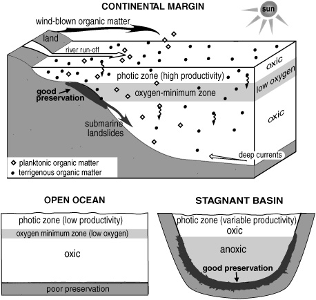
Organic geochemists observed in the early 1970s that the relative amount of pristane and phytane in sediments seemed to be related to the amount of oxygen in the depositional environment, with more pristane than phytane in oxic environments and less pristane than phytane in anoxic ones. This fit with what the Bristol group was learning about the diagenesis of phytol, wherein a number of reaction pathways were likely to produce both pristane and phytane in the sediments—but all of the ones that produced pristane required oxygen, whereas those that produced phytane did not. In a first attempt at devising a proxy measure for past periods of water and sediment anoxia, they proposed that the ratio of pristane to phytane could be used as a rough indicator, with a ratio of less than 1.0 indicating an anoxic environment and anything greater than 3.0 signaling an environment where oxygen was readily available in the water and surface sediments. A number of factors besides oxygen availability may come into play, including the presence of other sources of pristane and phytane, but pristane–phytane ratios can indeed prove useful when taken together with other clues about depositional environments—including a number of similarly imperfect, but useful, biomarker proxies for anoxia.
In the presence of oxygen, the algal pigment fucoxanthin that is so abundant in diatoms is completely degraded and disappears without a trace, generating the more persistent loliolides only in thoroughly anoxic sediments. The presence of loliolides in some organic-matter–rich sediments from the Pleistocene thus indicates not only that diatom productivity was high, but also that the surface sediments or water had become anoxic.
The NIOZ group has suggested that gammacerane—among the first triterpenoids identified in the Green River shale and often abundant in sediments from highly saline environments—can be used as an indicator of highly stratified, partially anoxic water. Until recently, the only known sources of tetrahymanol, the presumed biological precursor to gammacerane, were the marine ciliates that tend to congregate at the sediment surface and other places where food is plentiful, eating anything small enough that falls into their paths. Ciliates happen to be easy to grow and manipulate in the lab, the unicellular equivalent of the biologist’s fruit fly, so quite a lot is known about their biochemistry—including the small detail that they produce tetrahymanol as a sort of surrogate sterol when, and only when, they can’t get sterols from their diet. The NIOZ group has reasoned that in highly stratified waters, the ciliates would feed mostly on the sterol-lacking bacteria that concentrate at the interface between the oxygen-containing surface water and the anoxic deep water. The story may, however, be more straightforward, as a number of other sources for tetrahymanol have recently been discovered, among them purple photosynthetic bacteria that can only live in anoxic environments.
Oxygen-shy bacteria do, in fact, provide a few explicit biomarkers for water column anoxia. Among the compounds that the Strasbourg group found during its explorations of the Paris Basin shales in the 1970s was isorenieratene, an unusual carotenoid pigment with aromatic rings at either end. Natural products chemists had isolated it from green sulfur bacteria—photosynthetic organisms that use sulfide instead of oxygen and employ special pigments that are sensitive to long wavelengths—which can thrive in the penumbra beneath the sunlit photic zone, up to 200 meters below the sea surface in clear waters. They require a thoroughly anoxic and sulfidic environment, and live in places like the Black Sea—where isorenieratene has been found in sediment trap material from the water column as well as in the sediments—and, apparently, the shallow sea that once covered the region around Paris. Oil-producing shales commonly form in such environments, where organic matter is both plentiful and well-preserved, and in the late 1980s, Roger Summons, working at Australia’s now-defunct Baas Becking Geobiological Laboratory, identified isorenieratane and other reduced versions of the pigments in ancient crude oils. Green sulfur bacteria also contain a unique set of chlorophyll pigments, with characteristic patterns of side chains attached to the central chlorin ring system—patterns that Maxwell’s student Kliti Grice found preserved in the ancient rocks she was studying in the 1990s. She determined the structures of the nitrogen-bearing ring fragments of chlorins, produced by its oxidation in the laboratory and, apparently, in the sediments—structures called maleimides that included one with a distinct isobutyl sidechain found only in the bacteriochlorophyll e made by green sulfur bacteria. The green sulfur bacteria thus announce their passing quite unambiguously, which is very convenient, given their specific needs: the presence of isorenieratene, or the closely related chlorobactene—or their reduced fossil versions—or of the unique methyl isobutyl maleimide that Grice identified clearly indicates that the water was anoxic up to a couple hundred meters from the surface at the time of sediment deposition.
Determining how much oxygen was present in the sediments beneath the oxic waters typical of most marine settings is somewhat more problematic—and yet crucial to understanding past changes in primary productivity, organic matter preservation, deep sea circulation, and climate on a global scale. The most promising techniques to date make use of pairs of biomarkers that differ markedly in stability under oxic conditions, and either come from the same sources or have had a constant rate of input to the sediments over the period studied. Joan Grimalt and his Barcelona cohort used the ratio of C18 unsaturated to C18 saturated fatty acids to compare the oxicity of Pleistocene sediments deposited at different times and places, taking advantage of the knowledge that unsaturated fatty acids decompose faster than their saturated counterparts in the presence of oxygen. Long-chain alcohols break down more rapidly than the corresponding n-alkanes and have a common source in the leaf waxes, so the ratio of C26 or C28 n-alkanol to C29 n-alkane has provided an even more reliable measure of changing oxicity and decomposition rates in areas with significant inputs from the continents.
Researchers have long noted relatively high concentrations of the 40-carbon acyclic isoprenoid lycopane in sediments, rocks, and oils from anoxic environments, and have attempted to use it as an empirical measure of changes in sediment oxicity, though it’s unclear exactly where the compound comes from. A highly unsaturated analogue, lycopene, is a common component of the carotenoid pigments in algae and cyanobacteria, and there is some evidence that lycopane or its precursor comes from oxygen-requiring photosynthetic organisms. Possibly, lycopane is relatively abundant in anoxic environments because its unsaturated precursor breaks down rapidly when oxygen is present and there simply isn’t enough time for it to be reduced and preserved.
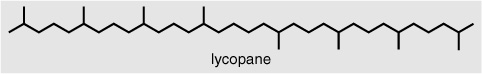
The NIOZ group, together with Jürgen and Sonja Schulte in the Oldenburg lab, studied the surface sediments beneath upwelling zones in the Arabian Sea and off the coast of Peru and found that the ratio of lycopane to the resistant C31 n-alkane accurately reflected the degree of oxygen depletion in the sediments, suggesting that the lycopane/C31 n-alkane ratio might be used as an oxicity index for ancient environments if one could gauge variations in the input of the two compounds.
Though there is clearly no single, reliable quantitative way to measure the history of marine productivity, oxicity in the sediments, and the export of carbon from the atmosphere to the deep water and sediments, multiproxy studies that include an array of biomarkers and mineral or paleontological indicators are beginning to provide qualitative records of many aspects of climate and associated ecosystem change over the past few million years. There is a certain opportunistic element to these studies, as they require sediments that can be dated reasonably accurately and that contain a relatively large amount of organic matter. A number of studies have focused on the thick, organic-matter–rich sediments deposited in the anoxic Cariaco Basin over the course of the last glacial to interglacial shift. Analysis of the algal biomarkers indicates that the last and most severe of the abrupt climate changes to interrupt warming about 11,000 years ago, the Younger Dryas, had a marked effect on primary productivity even in this tropical region. Concentrations of dinosterol, brassicasterol, fucosterol, β-sitosterol, cholesterol, and C37 alkenones all spiked at this time, indicating a transient increase in productivity that was in keeping with the changes in the tropical wind system and increased upwelling during the thousand-year cold snap. But the event also seems to have marked an enduring shift in the structure of the phytoplankton community, because the relative proportions of these compounds shifted dramatically, and irreversibly, with diatoms dominating during the Younger Dryas and coccolithophores and dinoflagellates taking charge for the rest of the Holocene.
Temperature proxy records in sediments and ice indicate that the last glacial period, from 50,000 to 20,000 years ago, was punctuated by numerous abrupt climate changes. At a subtropical site in the western Atlantic, Grimalt and his coworkers found that the accumulation rate of both n-alkanols and n-alkanes exhibited a pattern of abrupt change that was closely correlated with sea surface temperature changes, with the leaf wax compounds increasing during the cold spells—putative evidence that the northwesterly winds had abruptly increased in intensity, bringing more dust from North America. The relative amounts of alkanol and alkane didn’t change, indicating that the rate of decomposition and amount of oxygen in the water and sediments at this open ocean Atlantic site had remained constant. But in sediments from the western Mediterranean, the ratio of alkanol to alkane fluctuated in beat with the climate changes, decreasing during the cold snaps—evidence, according to Grimalt and crew, that these events involved influxes of cold, oxygen-rich Atlantic deep water into the Mediterranean.
Meixun Zhao, Geoff, and their colleagues at Dartmouth College and Bristol studied sediment sequences spanning the past 160,000 years and two glacial cycles at a site in one of the upwelling zones off the Atlantic coast of northern Africa, near Cap Blanc. Large fluctuations in the accumulation of chlorin marked dramatic changes in overall productivity, and changes in the relative amounts of dinosterol, alkenones, alkane diols, and silica showed that the structure of the phytoplankton community had varied significantly. But the group was hard-put to discern the relationships between these changes and the changing climate regimes. There was no correlation with sea surface temperatures, so changes in the intensity of upwelling, which brings nutrients and cold water to the surface, were not, apparently, responsible. Productivity did vary with the amounts of leaf wax n-alkanes and n-alkanols, presumably because the phytoplankton were stimulated by nutrients from minerals in the dust and river runoff that carried them. Geoff says he’d often noted that increases in alkenone content in Atlantic sediments coincided with increases in leaf wax n-alkanes, presumably for the same reason. But at a coastal site like the one at Cap Blanc, the changing inputs of leaf wax compounds could be reflecting any of a number of climatic factors: simple changes in the intensity of the dust-carrying winds; shifting weather patterns that produced more rain in certain regions on the continent and more runoff into the ocean; or the opposite, increasing aridity or a change in wind direction so that winds came from a more arid region and picked up more dust.
The biological pump hypothesis maintains that relatively high rates of marine productivity in key regions of the world’s oceans might have been responsible for lowering the concentration of atmospheric CO2 during glacial periods, as recorded in the ice cores. An alternative hypothesis suggests that the structure of the phytoplankton community may have shifted in favor of coccolithophores during the warm periods, and formation of their calcium carbonate coccoliths would have liberated CO2 to the water and atmosphere. Evidence for or against either hypothesis has been elusive, and one might hope that these detailed histories of marine primary productivity in various parts of the globe would provide some enlightenment. But neither the changes in productivity nor the variations in the structure of the phytoplankton community at the Cap Blanc site showed correlations with global climate patterns. Similar studies of sediments from the Indian Ocean and Arabian Sea indicate that in these areas the amount of productivity and the structure of the phytoplankton community both remained relatively constant over the past two ice age cycles. Analysis of the chlorins in a core from the South China Sea, northwest of Taiwan, revealed clear oscillations in the overall productivity of phytoplankton that were apparently related to oscillations in the intensity of the winter monsoon season in the region, with productivity at its highest toward the end of the last glacial period, at the onset of warming. Clearly, such studies are still too few and too incoherent to be integrated into geochemists’ models of the global carbon cycle—and, for various reasons, the organic geochemists may be looking in the wrong places.
One region where changes in the intensity of the biological pump might have had a concerted effect on the concentration of atmospheric CO2 during glacial periods is in the Southern Ocean encircling Antarctica, where, in the current interglacial period, the major nutrients, nitrogen and phosphate, are readily available and primary productivity appears to be limited by a lack of micronutrients such as iron—which might well have been supplied by additional inputs of wind-borne dust from the South American pampas, Africa, or Australia during glacial periods. This is a difficult region for oceanographic cruises, however, and appropriate sediment cores have been relatively hard to come by. One of the few multiproxy biomarker studies was done by a couple of Grimalt’s former students, working with the group that Roger Summons had helped build in Australia. They analyzed sediment cores from the Tasman Sea, south of Australia, determining concentrations of long-chain n-alkanes, brassicasterol, dinosterol, and alkenones in sediments deposited over the last 350,000 years. The concentration of n-alkanes at this site clearly fluctuated in concert with the glacial–interglacial cycles and correlated with the content of dust trapped in the Antarctic ice cores, increasing during glacial and decreasing during interglacial periods. Dinosterol and brassicasterol show a positive correlation with the Milankovitch cycles and the n-alkanes, but the alkenones show none. The brassicasterol fluctuations are particularly pronounced, and the authors postulate that silica in the dust may have given the diatoms a particular advantage during glacial periods. They propose that the high productivity of diatoms and dinoflagellates, specifically, during the glacial periods—and not of coccolithophores, whose calcium carbonate shells would have liberated CO2 and countered the effects of enhanced organic matter production—provides nominal evidence that the biological pump was operating in the hypothesized manner in this key region, and may indeed have played a significant role in regulating the fluctuations in atmospheric CO2. But, of course, such studies are still just a drop in the bucket of evidence needed to reconstruct and understand the patterns of cause, effect, and feedback that comprise the earth’s climate history on a global scale.
Most multiproxy biomarker studies have focused on sediments that are particularly rich in organic matter, for the obvious reasons that the organic compounds are better preserved and more easily detected. But such sediments often pose a mystery in and of themselves. Sediment cores from the Mediterranean Sea exhibit bands of black, organic-matter–rich sediments periodically interspersed in pale brown and yellow sediments with less than 0.1% organic matter. From a few centimeters to a few decimeters thick, spanning up to 10,000 years and containing up to 30% organic matter, these black sediments, which geochemists call sapropels, began appearing about five million years ago, during the early Pliocene when the first ice sheets were forming in the northern hemisphere. There must have been drastic, periodic changes in the Mediterranean environment to produce them—but what?
A lack of fossils from bottom-dwelling foraminifera hinted that oxygen may have been lacking in the surface sediments and deep water of the basin, and recent biomarker analyses offer more evidence: loliolides are abundant, and in at least two of the Pliocene sapropels, isorenieratene is present, implying that the anoxia extended into the lower photic zone, as in the contemporary Black Sea. Had circulation in the Mediterranean somehow changed? Was it shut off from the Atlantic? Or did the input of organic matter suddenly increase so dramatically that all the oxygen in the deep water was used up by decaying organic matter? An increase in the ratio of long-chain n-alkanols to n-alkanes within the sapropels indicates that preservation of organic matter increased significantly during the shift from an oxic to an anoxic environment, as might be expected. Dramatic increases in the accumulation rates of organic matter, and of phytoplankton biomarkers such as loliolide, brassicasterol, alkenones, alkane diols, and dinosterol, are also observed and must, to some extent, be the result of enhanced preservation. But there are also indications that primary productivity increased, and the greater diversity of phytoplankton biomarkers within the sapropels reflects a more diverse community, as is generally observed when primary productivity is high. An increase in the absolute amounts of leaf wax n-alkanes signals an increase in the input of material from land, with its associated nutrients, which would have fueled phyto-plankton growth. And in at least one of the sapropels, the chain-length distribution of the leaf wax n-alkanes shifts to shorter chain lengths, implying that they came from vegetation growing in a more humid region.
Mediterranean sapropels: the biomarker story (mid-Pleistocene period)
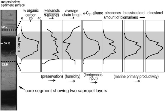
The emerging story, based on these and other chemical and geologic data, is that a periodic intensification of the monsoon system and more precipitation in Europe and Africa—in sync with the earth’s 23,000-year cycle of precession on its spin axis—brought more river runoff and nutrients into the Mediterranean, spurring phytoplankton growth, an excess of organic matter production, decomposition, and anoxia, and resulting in the periodic deposition of the sapropels. That all makes a fine story for the Mediterranean, which is a restricted basin where a few nutrients and a little extra organic matter production go a long way … but some of the first DSDP cores in the 1970s had revealed that, some hundred million years earlier, similar layers were deposited in the middle of the open ocean.
Like the Mediterranean sapropels, the Cretaceous black shales appear as dark bands of organic-matter–rich sediment in the midst of long stretches of pale gray or white mudstones and limestone. Laminations in the sediments and the sudden disappearance of fossils of bottom-dwelling foraminifera indicate that oxygen in the bottom water was in short supply. But these black shales were deposited over longer stretches of time, with no apparent pattern in the timing, between 140 and 80 million years ago. Most remarkably, they appear contemporaneously in cores drilled thousands of miles apart in areas of the world’s oceans where it is hard to conceive how so much organic matter could possibly have accumulated. Five such sediment layers have now been identified in the middle and late Cretaceous, and one way back in the early Jurassic period. They present an even greater enigma than the Mediterranean sapropels, manifesting episodic perturbations in the chemistry and biology of the world’s ocean—which oceanographers initially dubbed “oceanic anoxic events”—that lasted from a few hundred thousand to more than two million years.
The biomarkers in these black shales tell a story of anoxia that may have been almost as severe as that in the present-day Cariaco Basin or Black Sea—but on an oceanwide scale. High concentrations of lycopane and steroids relative to long-chain n-alkanes and a low ratio of pristane to phytane corroborate other evidence that oxygen was in low supply in the sediments and deep water of the Atlantic during these anoxic events. But the NIOZ group and others have also found significant concentrations of isorenieratane and other molecular fossils of isorenieratene and chlorobactene in black shales from at least two of the events, and the Bristol group has found the telltale isobutyl maleimides and related porphyrins—all indications that green sulfur bacteria were thriving.
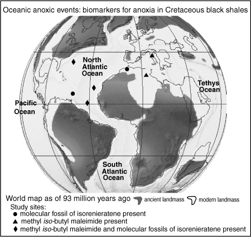
Either the deep water was entirely anoxic from the sediments to within 200 meters of the surface, or there was a mid-depth zone of decomposition, an oxygen-minimum layer that was entirely anoxic, as in parts of the contemporary Arabian Sea. Of course, the oceans and continents looked very different during the Cretaceous than they do today: the Atlantic Ocean was still a relatively young, narrow waterway, recently formed by seafloor spreading, and the ancient Tethys Ocean on the other side of Africa was shrinking. It’s easy to imagine these oceans with obstacles to the circulation needed to replenish oxygen in their deep water, or so shallow that the bottom of the photic zone coincided with the sediment surface and made for a particularly intense zone of microbial activity and oxygen consumption. Relatively low concentrations of leaf wax n-alkanes and the absence of oleanene or oleanane indicate that little of the organic matter came from the continents, while high concentrations of HBIs and of 27- and 28-carbon steroids attest to a particularly productive phytoplankton community. In the Atlantic and Tethys oceans, at least, it would seem that a spurt in marine productivity generated enough additional organic matter and oxygen- consuming decomposition to send a warm, nearly stagnant and stratified ocean over the edge into a state of anoxia that, in modern times, exists only in a handful of isolated basins. But black shales are also found in the Pacific Ocean, which by all accounts was a vast, largely unencumbered expanse of water during Cretaceous times. In recent studies of black shales deposited in the middle of the Pacific about 120 million years ago, Simon Brassell’s group, now at Indiana University, found low ratios of pristane to phytane and relatively high lycopane concentrations, implying that low-oxygen conditions, if not photic zone anoxia, may have existed during this event even in the open ocean. Had the Pacific Ocean also stagnated? Or could marine productivity have increased so drastically, for such extended periods, around the entire globe? And, most problematic of all, why and how?
There always seems to be something missing in these multiproxy studies, yet another parameter that will constrain the others—a mineral that no one has the wherewithal to analyze, or the particular biomarker that couldn’t be analyzed because it is too difficult to separate on the GC column used or because the student doing the project ran out of time; or perhaps some crucial bit of sediment core got lost during the coring operations, or worms in the sediment had mixed up the layers during or shortly after deposition and the time periods were not well resolved.… Perhaps if these organic geochemists had gotten a few more data points beyond the juicy black shales and sapropels they’re so fond of, or had pushed their analytical techniques to the max and provided information about the biomarker composition of the 0.1% organic matter in the mudstone that was deposited during the 5,000 years before and after, or if they had moved away from their favorite coastal upwelling sites and analyzed the Pleistocene sediments from the places that paleoceanographers and climatologists consider key to understanding the global cycles of nutrients and primary productivity … The problem, of course, is that the organic matter is so poorly preserved in these well-oxygenated, open ocean areas that what one finds is not at all representative of the overall biological input and may not be particularly informative—but the cumulative data from such sites may be. Eloquent simplicity is not necessarily a forte when it comes to using biomarkers in paleoenvironmental studies. Rather, “the more the merrier” would seem to be the better guiding principle, the full exploitation of the expanding molecular lexicon and increasing instrumental sensitivity—along with appropriate statistical treatments and comparative ratios to turn the jumble of data produced into meaningful parameters that can be integrated into the larger context of paleoceanographic and paleoclimate studies. But first, we must consider another dimension of molecular information, one that started adding ballast to the lexicon in the 1980s and would eventually promote the interpretation of biomarker data to a higher art.