The limits of my language, mean the limits of my world.
—Ludwig Wittgenstein, 1889–1951, Austrian philosopher From Tractatus Logico-Philosophicus (1921)
The attitude of man towards the earth is still, on the whole, that of a parasite. For a parasite, nevertheless, the life of the host is of prime importance.
— Lourens G. M. Baas Becking, 1895–1963, biologist and inventor of the term “geobiology”
Quoted in Anton Quispel, International Microbiology 1 (1998)
Throughout the 1980s, while the molecule collectors were busy exploring the ocean sediments, tracking their finds into the past, and learning to read the messages hidden in the carbon skeletons, one analytical chemist cum geochemist at Indiana University was finding that important elements of the lexicon lay not only in the molecular structures, stereochemistry, and distributions of the carbon skeletons, but in the carbon atoms themselves.
John Hayes had done his graduate work at MIT in the mid-1960s under Klaus Biemann, one of the doyens of mass spectrometry who, like Carl Djerassi, was interested in natural products with biomedical applications. When Hayes told Biemann he wanted to do his doctoral thesis on the organic constituents in meteorites, Biemann was uninterested, to say the least. Forty years later, Hayes can still quote the eminent scientist’s response to his proposal, replete with thick Austrian accent: “Don’t talk to me about zat junk.” Biemann walked away from the discussion without another word, and Hayes was so mortified by his own foolishness that he couldn’t bring himself to tell his wife about the incident. When he went into the lab the next day, he was convinced that his graduate career was over—but Biemann had done some homework and had a change of heart. “It seems we can get lots of money for zat junk!” he exclaimed as soon as he saw Hayes. NASA was, at the time, offering generous funding for such projects.
For all his skepticism, Biemann was eventually seduced by the extraterrestrial “junk” and even ended up designing the mass spectrometer for the Viking Mars mission. Hayes remembers him commenting, a couple of years into the meteorite project, that it was actually “much more interesting than the thousandth alkaloid in the thousandth tree,” though Hayes himself says his doctoral thesis was unexceptional, completed before the Murchison meteorite fell and things really got interesting. While he was working on it, however, struggling to divine how and where the organic compounds he detected in his samples had formed, he had an idea that would, years later, form the catalyst for some of his most remarkable accomplishments: it occurred to him that the carbon atoms themselves should bear witness to a molecule’s provenance.
As Hayes tells the story, the idea began to evolve during the countless hours he spent staring at the forests of little black lines, the so-called “peaks,” in countless mass spectra. There were the peaks of interest, corresponding to the molecular ion and fragment ions generated when the molecule was hit by an electron and broken up. But lined up on the heavy side of each of these main peaks was a minority population of little ones, corresponding to the same ion but containing one or more atoms of the rare heavier isotope of carbon. In the early days of organic mass spectroscopy, the spectra submitted for publication were often cleaned up to remove the black fur of peaks produced by traces of impurities in the sample, occasionally even doctored to the point that the isotope peaks disappeared and only the “useful” peaks remained. Anyone who worked with mass spectroscopy on a regular basis, however, knew that no naturally occurring substance, even an absolutely pure one, could generate such a clean spectrum. For his part, Hayes spent so many long hours communing with “real,” undoctored mass spectra that he decided the messy isotope peaks must be “good for something” in their own right.
Naturally occurring heavy versions of most of the elements that make up organic compounds—carbon, hydrogen, oxygen, nitrogen, and sulfur—had been identified in the 1920s and 1930s. Generated by the nuclear reactions within stars and inherent to the elemental makeup of the planet, they comprise a small percentage of these elements’ total inventories on Earth: 0.02% of oxygen is 18O, and the heavier 13C isotope comprises 1.1% of the earth’s inventory of carbon. These scarce heavy isotopes have an extra neutron or two in their nuclei but the same number of protons as 16O or 12C, and they are involved in all the same reactions as their mainstream counterparts. But the slight difference in mass makes for slight diff erences in the ease with which a given physical or chemical process occurs in molecules containing diff erent isotopes, resulting in the isotopes being preferentially distributed or fractionated between diff erent substances. With the development of mass spectrometers capable of accurately quantifying small diff erences in the abundance of these atoms, it became possible to observe the effects of this fractionation over the course of earth history.
The isotopes of a given element are not evenly distributed between diff erent materials, but, rather, ice and snow are depleted in 18O relative to seawater (the reason the ice ages had such a pronounced eff ect on the δ18O of foraminifera), plants and organic-matter–rich rocks are depleted in 13C relative to carbonate rocks, and so forth. Some of these diff erences can be predicted directly from the fundamental physical and thermodynamic properties of the atoms: a chemical bond to a heavier isotope has a lower vibrational energy and is ever-so-slightly stronger than a bond to its lighter counterpart; molecules containing a heavy isotope usually react more slowly in chemical reactions than their lighter versions do; and in a reversible reaction at equilibrium, the heavier isotope is concentrated in the compound where it is bound most strongly. These theoretical considerations account for the observations that water containing 18O evaporates less readily than the usual H216O does, and the bicarbonate in seawater is enriched in 13C compared to the dissolved carbon dioxide.
The ratio of 13C to 12C in biologically produced organic molecules depends on the ratio of 13C to 12C in the material that provided their carbon atoms and on any isotope fractionation that occurs during their assembly and should, in principle, diff er from one compound to the next and from one environment to the other. Indeed, Phil Abelson and Thomas Hoering did experiments with amino acids at the Carnegie Institute in 1961 and showed that 13C was distributed unevenly even within the same compound. John Hayes was impressed when he read their paper as a student: presumably, the diff erent steps in the biosynthesis of organic compounds involved varying degrees of fractionation, and this was registered by the distribution of 13C. Some positions in the molecule must be more enriched in 13C than others, and the little isotope peaks in the molecule’s mass spectrum should, in principle, show this! They were good for something! If you could measure the ratio between the isotope peak and the main peak for each of a molecule’s fragment ions, then you could figure out the precise distributions of isotopes in any organic molecule you could analyze by GC-MS. And if one could determine the precise distribution of isotopes in the organic compounds in an extract from a meteorite or Precambrian rock, then one would have a very specific record of where and how those organic compounds had formed—the question of the day.
It was a naive proposition, a student’s fantasy—not much was known about isotope fractionation during specific biosynthetic reactions, and one could not, even with Klaus Biemann’s sophisticated array of mass spectrometers, detect the minute diff erences in the sizes of the fragment ion isotope peaks. Nevertheless, Geoff says that when Hayes was in Bristol as a postdoc, his idea that one could, in principle, determine the precise isotopic makeup of individual compounds was the subject of many long conversations—not in connection with the lunar samples they were analyzing at the time but, rather, with the homely old leaf wax hydrocarbons. True to form, Geoff was enthusiastic and encouraging: if one could determine the isotopic makeup of the n-alkanes extracted from sediments, it would add a whole new layer of information as to their origins, maybe even the conditions under which they were biosynthesized!
Warren Meinschein, who had finally answered the call of academic science and left Esso, was likewise interested, and when Hayes joined him at Indiana University in 1970, they made a first attempt to develop the idea. Hayes approached the engineers at the Finnigan-MAT instrument company in Germany about designing a new instrument, and they began what would turn out to be a career-long collaboration—despite the nominal failure of their first enterprise. Hayes has a vivid memory of spending Thanksgiving Day 1972 in the lab eagerly trying out the new prototype from Germany … only to discover that his grand experiment, if not the instrument itself, was a total failure. The instrument combined the precision of the isotope ratio mass spectrometers used by geologists to analyze carbonates with the capabilities of the mass spectrometers used by organic chemists. It was supposed to allow determination of 13C to 12C ratios for each of a molecule’s fragment ions—but there were unforeseen problems with hydrogen atoms moving around when the molecules fragmented, and the isotope ratios were variable and unreliable.
Discouraged but not dissuaded, Hayes resorted to dismantling the molecules chemically, carbon atom by carbon atom, and using the new mass spectrometer to measure the isotopic composition of each piece. The method was useless for geochemical samples, but it did eventually reveal the distinct isotopic composition of a fatty acid molecule. And it did, in turn, inspire a fascinating medley of investigations into the various biosynthetic processes responsible for distributing the isotopes of carbon both within and among organic molecules. Pat Parker and his team of microbiologists in Texas, plant physiologists and biophysicists in Australia and California, and geochemically inspired biochemists in Japan, not to mention Hayes’s own group in Indiana, all contributed bits of insight.
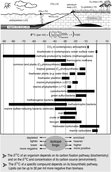
The carbon isotope composition of a material is generally expressed as “δ13C,” defined as the amount that the 13C to12C ratio measured in a substance deviates from that of the CO2 generated by dissolving an international calcium carbonate standard—originally from a rock formation in South Carolina—expressed in parts per thousand (per mil or 0/00). It is, however, not the δ13C values per se that are of interest, but comparisons of isotopic compositions of diff erent materials, the diff erences between δ13C values in the various components of a system: between the diff erent kinds of molecules in a cell, or between the organisms in an ecosystem and their inorganic carbon sources, or between the various carbon-containing components of a geologic deposit—between carbonate rocks and bulk organic matter, or between specific fossil molecules in the organic matter.
As Hayes showed with his fatty acid dismantling experiments, biological isotope fractionation can occur during each step of a biosynthetic process. This results in the uneven distribution of isotopes within molecules, and it creates significant diff erences in the overall isotopic compositions of diff erent classes of molecules. In algae, for example, the sugars generated directly by photosynthesis are generally less depleted in 13C than the lipids are, with diff erences ranging from 2 to 10 per mil, depending on the species and the specific compounds; isoprenoid lipids tend to be slightly less depleted than n-alkyl lipids; and so forth. The most pronounced carbon isotope fractionation in biology, however, one that is registered in the δ13C values of an organism’s entire biomass, generally occurs during the initial transfer of carbon from geosphere to biosphere. Plants, algae, and microorganisms all exhibit a preference for the lighter, 12C-containing version of their carbon sources—carbon dioxide or bicarbonate for photosynthetic organisms, or methane for certain methanotrophic microorganisms. Thus a plant will be significantly depleted in 13C relative to the CO2 in the air—more than 20 per mil in the case of some land plants—and an alga will be depleted relative to the dissolved CO2 or bicarbonate in the water where it grows, and so on. Moving up the food chain to animals and other heterotrophic organisms that use biologically prefabricated organic matter as their carbon source, the fractionation goes in the opposite direction: as organic matter is respired and burned to CO2, carbon–carbon bonds are being broken and 12C is released more readily than 13C. Thus the compounds in heterotrophic organisms will generally be slightly enriched in 13C relative to their food sources, with each step up the food chain resulting in about 1–1.5 per mil enrichment compared to the one before it.
By the mid-1980s, many of the details of biological isotope fractionation that Abelson and Hoering, John Hayes, and others had only been able to theorize about in the 1960s were documented, and it was apparent that the isotopic composition of fossil molecules might provide precisely the sort of information Hayes had imagined as a starry-eyed graduate student, even without resort to the intramolecular details. Limited at first to fossil molecules that could be isolated and purified—the most plentiful compounds in the most organic-matter–rich rocks—Hayes teamed up with Pierre Albrecht in a study of the Strasbourg group’s favorite rock, the Messel shale. The group in Strasbourg extracted and purified the compounds, determined their molecular structures, and sent them to Hayes in Indiana. Hayes and his students burned each compound and injected the CO2 gas produced into a conventional isotope ratio mass spectrometer to determine its 13C content—much as oceanographers did when they determined the δ13C of bulk organic matter. Hayes says he had some exceptional students around this time— Kate Freeman in particular, he claims, was blessed with “golden fingers”—and it wasn’t long before the researchers contrived an interface that allowed them to connect a gas chromatograph directly to an isotope ratio mass spectrometer. As each compound emerged from the GC column, it was converted to a puff of CO2 and fed directly into the mass spectrometer, where its 13C content could be determined on the fly, so to speak. They called the technique gas chromatography– isotope ratio monitoring–mass spectrometry, which quickly reduced to the acronym GC-irm-MS. With it, they could determine the isotopic composition of any compound in a mixture that could be cleanly separated on a GC column.
The Indiana-Strasbourg Messel shale studies of the late 1980s illuminated the full potential of compound-specific isotopic information to elucidate the ecology of an ancient ecosystem, in this case a large lake during the Eocene epoch. The Strasbourg group had identified the structures of more than a dozen porphyrins, some of which clearly derived from algal chlorophylls or one of the bacteriochlorophylls, and some of which were of ambiguous origin. The δ13C values of the bacteriochlorophylls were consistently 2 per mil more negative than those of the algal chlorophylls, and the δ13C values for most of the ambiguous porphyrins bore the distinct signature of one or the other, allowing their tentative assignment to bacterial or algal sources. The δ13C of dinosterol was slightly more depleted than that of the algal porphyrins, reflecting the diff erent biosynthetic pathways that presumably linked them to a common source of CO2 in the surface water. Isoarborinol, a triterpenol found exclusively in land plants, had a δ13C very similar to that of contemporary land plants, and visible fossils in the shale indicated that organic matter from higher plants had made a significant contribution to the sediments, apparently washing into the lake from the surrounding watershed. None of the porphyrins, however, had a δ13C within the range expected for land plants, which supported the hypothesis that land plant chlorins were unable to survive the exposure to oxygen during the journey from land to lake sediment.
Typical δ13C values in organisms, the environment, and geologic deposits
One long-chain acyclic isoprenoid structure that was present in high concentrations in the Messel shale had recently been linked to the unusual membrane lipids of methanogenic microorganisms, which required completely anoxic conditions and were often found deep in the sediments. These methanogens obtained their energy by reducing CO2 or acetic acid to methane, a process which involved one of the largest carbon isotope fractionations in nature: the methane produced in laboratory experiments with the organisms was 40–95 per mil more depleted in 13C than the CO2 or acetate that the organisms imbibed. Fractionation during the assimilation of carbon for molecule-building purposes was apparently more moderate, however, and the methanogens themselves were only slightly more 13C depleted than photosynthetic algae grown from the same carbon source. Of course, in a place like the Messel Lake, methanogens and algae weren’t likely to have used the same carbon source, because the algae lived near the lake surface, using CO2 that was equilibrated with the air, whereas methanogens could only have lived in the anoxic environments deeper in the lake or sediments, using the 13C-depleted CO2 or acetate generated by decomposition of organic matter. In the shale, Hayes and crew found that the unusual long-chain isoprenoid was about 8 per mil more depleted in 13C than pristane, whose δ13C value matched that of the algal lipids. They inferred that the pristane had come from the decomposition of chlorophyll, whereas the long-chain isoprenoid and most of the phytane—which was similarly depleted in 13C and seemed to be a likely diagenetic product of the newly identified methanogen lipids—derived from methanogens. Remarkably, two other long-chain acyclic isoprenoids and several of the hopanoids were so depleted in 13C, with δ values ranging from –60 to –75 per mil, that they seemed to have been made by organisms that used the methane released by the methanogens. Precisely what those organisms were and the amazing ways they operated would not be apparent for more than a decade, but the distribution of porphyrins implied that green sulfur bacteria may have been present and the lake water anoxic, which meant that methane could have been produced throughout much of the water column, as well as in the sediments.
The most significant revelation of the Indiana-Strasbourg team’s studies in the 1980s resulted from their comparison of the δ13C values for the individual microbial and algal biomarkers—the hopanoids, acyclic isoprenoids, steroids, and porphyrins—with the δ13C of the bulk organic matter, both kerogen and bitumen, in the shale. Despite the rich, diverse flora and fauna that apparently lived in and around the ancient Messel Lake and left such well-preserved fossils for posterity, the supreme rulers of the lake’s ecology and regulators of the flow of carbon and dissolved gases within its margins were, in fact, the heretofore invisible microbes.
Another geochemist who was becoming acutely aware of the pivotal role that microbes played in the movements of carbon through the biosphere and geosphere, and who, like Hayes, had been thinking about putting the isotopic dimension of fossil molecules to use in understanding it, was Roger Summons in Australia. Summons had spent the early years of his career studying biochemical processes in plants, and his first forays into organic geochemistry were under the auspices of the Baas Becking Geobiological Laboratory—Australia’s homage to one of the first microbiologists to recognize the importance of microbial life in regulating geochemical cycles and forming geologic deposits. In the 1970s and 1980s, the Baas Becking Laboratory was one of the few places in the world where geochemists and microbiologists worked side by side on the same fundamental research questions. Even before Hayes and crew started their compound-specific isotope measurements on the Messel shale porphyrins, Summons was painstakingly isolating what appeared to be fossil remnants of isorenieratene from crude oil samples, determining their isotopic makeup, and noting that they were distinctly enriched in 13C. He happened to be aware of recent biochemical studies showing that green sulfur bacteria not only employed a sulfur-based version of photosynthesis and contained unusual carotenoid pigments, but also captured CO2 via a unique sequence of reactions that resulted in relatively little carbon isotope fractionation and created a biomass that was enriched in 13C relative to that of most other phytoplankton. The isorenieratane in the crude oils was 8 per mil enriched in 13C compared to the other hydrocarbons in the oils, putative proof of the compound’s provenance from the green sulfur bacteria carotenoid—and of the oils’ provenance from source rocks formed in an anoxic depositional environment. It was the first so-called compound-specific isotope analysis, in which the distinct isotopic signature of a source organism’s biochemical system was used to track the origin of a fossil molecule—something that Hayes’s new GC-irm-MS would soon make possible for tiny traces of compounds that couldn’t be readily isolated.
In 1988, as the Indiana group was beginning its first explorations with its new instrument, Hayes arranged to spend his Guggenheim fellowship in Summons’s lab in Australia, initiating years of collaborative isotopic explorations and establishing a tradition of trans-Pacific winter migrations for several generations of Indiana students. Ironically, that was the same year that the Baas Becking Geobiology Laboratory met its demise at the hands of Australian bureaucrats— just as geochemists and microbiologists in other parts of the world were beginning to recognize the value of disciplinary intermarriage. Summons ended up working for the petroleum-oriented Bureau of Mineral Resources, but managed to continue the studies he’d nurtured at Baas Becking, working with a carefully chosen, interdisciplinary collection of collaborators around the world. Despite the misguided perceptions of Australian bureaucrats in the late 1980s, interest in the coevolution of biochemical and geochemical systems was growing, not just among a few starry-eyed geochemists and microbiologists but throughout the international oceanographic and geologic communities—with a particular emphasis on understanding how the global carbon cycle had changed throughout earth history.
An increasing amount of evidence from the Ocean Drilling Program cores indicated that the distribution of carbon between atmosphere, ocean, biosphere, and rocks had changed significantly—and in concert with the climate—over the course of the past 200 million years. Geologists had noted that the amount of isotope fractionation between the carbonate and the bulk organic matter in Cretaceous period sediments and rocks was consistently greater than in recent times, and that the organic matter in Cretaceous sediments was some 5 per mil more depleted in 13C than that in more recent sediments. Was this due to some pervasive difference in ocean ecology, radically diff erent distributions of species, or the imprint of some yet undiscovered bacterial process? Or was it, as the geologists speculated, due to universally enhanced isotope fractionation by plants and algae during the Cretaceous?
Hayes and company found that porphyrins isolated from Cretaceous marine sediments were even more depleted in 13C than the bulk organic matter was—the opposite of the situation in more contemporary sediments and an indicator that the enhanced fractionation was broadly associated with phytoplankton, just as some geologists suspected. How and why were a little more difficult to discern. Most plants incorporate CO2 via the cycle of biochemical reactions that Melvin Calvin elucidated in the 1950s. Though a handful of other pathways have been discovered in bacteria, and in tropical grasses and plants, the Calvin cycle was the only pathway known in marine algae, and it seemed unlikely that a diff erent species distribution could have caused such a large change in isotope fractionation. There were, however, indications from both geochemical data and laboratory studies that the amount of fractionation during photosynthesis by algae and photosynthetic bacteria might depend on the concentration of CO2 in the water where they grew—specifically, that they might be more discriminating in their choice of isotopes when the CO2 concentration was high. One of the most plausible explanations for the Cretaceous period’s warm climate invoked a greenhouse eff ect from high levels of atmospheric CO2, and paleoceanographers had found some evidence of extensive volcanism, which might have released large amounts of CO2—but such evidence was circumstantial, at best, because there was no way to measure the atmospheric pressure of CO2 millions of years ago, no paleo-CO2 proxy on par with the δ18O climate proxy or the newly developed alkenone sea surface temperature proxy … or was there? If the δ13C of the organic matter in the rocks was low because algae responded to an excess of dissolved CO2 in the ocean surface waters, then perhaps that eff ect could be quantified or calibrated.
Hayes had toyed with this idea since the late 1970s, when he first started trying to analyze the isotopic makeup of organic molecules. His oceanographer friends were more than a little intrigued by the idea of a paleo-CO2 proxy, but not until 1985—when a friend at Columbia University mentioned an unpublished Ph.D. thesis he was an external examiner for in New Zealand—did it begin to seem at all plausible. A student at Waikato University had done a study on natural mixed populations of algae that he’d collected from lakes in New Zealand and grown in the laboratory under carefully controlled conditions. Bruce McCabe had measured the δ13C of the algal biomass and that of the dissolved CO2 they used, and then determined how the difference between the two varied as he changed the concentration of dissolved CO2 in the water. It was the first time anyone had documented a predictable quantitative relationship between the amount of fractionation by the algae and the amount of available CO2. Whether or not one could turn that relationship into a calibration that would hold for organisms that lived millions of years ago, under variable climates and conditions, remained to be seen. That the δ13C of organic molecules generated by photosynthesis depended on the CO2 concentration in the water was clear. But there were also indications that isotope fractionation depended on a number of other environmental and physiological factors.
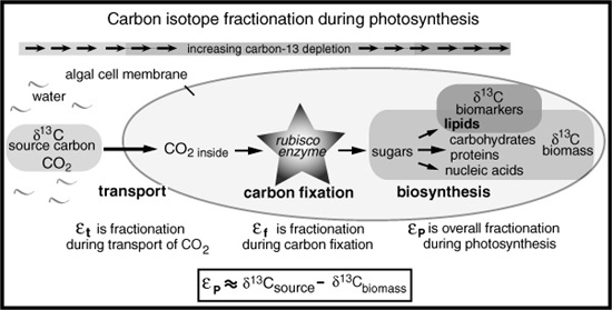
In Australia, the plant physiologist Graham Farquhar had just come up with a mathematical model for the isotope fractionation that accompanies uptake of CO2 during photosynthesis:
εP = εt + ([CO2]inside/[CO2])(εf − εt)
Here, the overall fractionation between the CO2 the plant or alga used and the organic matter produced by photosynthesis, εP, was expressed as a function of fractionation during the transport of CO2 across the cell membrane, εt; fractionation during the formation of the carbon–carbon bond as mediated by the carbon-fixing enzyme, εf; and the relative amounts of CO2 inside the cell, [CO2]inside, and in its environment, [CO2].
The marine algae and photosynthetic bacteria that live in the surface waters of the ocean use diff erent versions of the rubisco enzyme that fixes CO2, so they were likely to have diff erent fractionation factors, εf. In algae where CO2 moves into the cell by simple diff usion, the amount of fractionation εt and the concentration of CO2 inside the cell, [CO2]inside, might be predictable. But some algae complicate matters by actively transporting CO2 into their cells or making use of bicarbonate as well as dissolved CO2. And the concentration of CO2 inside the cell would also depend on growth rate, with fast-growing cells using it up faster and maintaining a lower concentration.
In his empirical calibration with the New Zealand lake algae, McCabe had simply found the best mathematical fit between the amount of CO2 in the environment and the amount of photosynthetic fractionation. If one wanted to use such an equation to determine the amount of CO2 in some other environment, one had to make the assumption—or hope—that the physiological factors that Farquhar had identified were either constant or had a relatively minor eff ect. The porphyrins that Hayes and Freeman had been analyzing in Cretaceous rocks were derived from chlorophylls made by a wide variety of photosynthetic organisms, but if one could determine δ13C values for a more specific biomarker, from a single species or group of algae, then this might not be such a bad assumption and one might indeed be able to estimate past levels of CO2. One would need the perfect biomarker, something particularly stable, from some extant group of algae with a long history and a wide distribution. And, of course, one would also need a way to determine the δ13C of the dissolved CO2 that the algae had imbibed.
In the summer of 1986, when Hayes presented his study of porphyrins in Cretaceous marine rocks at the Gordon Research Conference in New Hampshire, there was at least one Woods Hole graduate student in the audience who had been doing a lot of thinking about the “perfect biomarker.” The  index had hit the press earlier that year, and alkenones had been the talk of the town in Woods Hole—but John Jasper had been using them in his thesis research, even before the temperature proxy was developed. In comparing the changing inputs of organic matter in the Gulf of Mexico during glacial and interglacial periods, he had needed a relatively persistent, quantifiable index of specifically marine input, and the alkenones had won the prize hands down. Earlier that summer, Jasper and the other students had invited Geoff to Woods Hole for a special two-week seminar course, much of it spent in long, contemplative beach walks and seaside brainstorming sessions about other ways to use the new biomarkers. So as Jasper sat listening to Hayes talk about the relationship between CO2 and the amount of isotope fractionation by algae and plants, it was only natural that he should be thinking about the alkenones and his Gulf of Mexico core, which contained a very detailed record of glacial–interglacial climate change and was chock-full of alkenones.
If one could measure the δ13C of the alkenones and the δ13C of carbonate shells from planktonic forams, then one could determine a very explicit εP value from sediment extracts—specifically, for Emiliania huxleyi and a few closely related species of coccolithophores—avoiding most of the problems Hayes described. Jasper’s Gulf of Mexico cores covered 100,000 years, from the beginning of the last ice age to the present, and there was a good record of the CO2 content of the atmosphere for a portion of that period in the Greenland ice core. The ocean surface water was presumably in equilibrium with the air in most areas, and he would only need to know the temperatures, which he could obtain from δ18O or alkenone measurements, to determine the amount of CO2 dissolved in the water. He could then calibrate the relationship between εP and CO2 based on the alkenone δ13C measurements, and the changing concentrations of dissolved CO2 over the past glacial–interglacial cycle! Alkenones had been found in sediments dating back tens of millions of years, and though no one knew precisely what had made them then, one might assume that a limited number of closely related species of coccolithophore were also responsible. So one might, in theory, apply such a calibration to rocks dating all the way back to the Cretaceous … Jasper was so excited by these ideas that he went up to talk to Hayes right after the presentation. The problem, he admitted, was that he didn’t have any way of measuring the δ13C of alkenones in the complex mixtures he extracted from his sediments. But Hayes was enthusiastic—there was an instrument in his lab in Indiana that could do precisely that. They just needed to write a proposal so Jasper could work at Indiana University for a year or two when he finished his doctorate at Woods Hole.
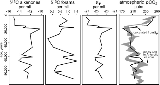
The initial results from the Gulf of Mexico core were exciting. Jasper measured the δ13C of the diunsaturated C37 alkenone and of the carbonate in foram shells from a single species known to live at approximately the same water depth as Emiliania. Alkenones are typically 3.8 per mil more depleted in 13C than the total biomass of the algae, so this amount was added to the alkenone δ13C to give values for the δ13C of the Emily biomass. The photosynthetic fractionation, εP, was then determined from the difference between the carbonate δ13C and the δ13C of the algal biomass. Jasper made a crude numerical calibration of the relationship between εP and CO2 concentration using a few of these εP measurements and dissolved CO2 concentrations calculated from the measurements of CO2 in the Greenland ice cores. He then used this calibration to calculate dissolved and atmospheric CO2 concentrations based on the εP values from the rest of his core samples. While he was working on the project, analyses of the CO2 content of air trapped in the long Antarctic ice core had been published, enabling a comparison between his entire 100,000-year alkenone proxy record of CO2 from the sediments and the record from ice core measurements.
Like the first appearance of the alkenone paleothermometer a few years earlier, the alkenone paleobarometer caused a stir when the first results appeared in Nature in 1990. The sawtooth pattern of the ice ages and the correlation between the glacial–interglacial shift and the amount of CO2 in the atmosphere were as apparent in the alkenone δ13C data as they were in the direct measurements of CO2 in the air bubbles trapped in the ice core. Some diff erences were also apparent, but their significance was yet unclear. The calibration itself was still crude, and the correlation between dates in the layers of ice and sediments was imperfect. Also, comparison of atmospheric CO2 measurements, as measured in the air from the ice cores, with dissolved CO2 measurements in the surface water, as recorded by the alkenones, assumed that the CO2 in atmosphere and surface water were in equilibrium—but occasional upwelling of CO2-rich deep water at the Gulf of Mexico site might have disturbed that equilibrium. In fact, one of the beauties of the method was that analysis of cores spanning the same time period in diff erent geographic locations might distinguish regional anomalies in the dissolved CO2 concentration of the surface ocean and determine where it had been out of equilibrium, either burping CO2 into the atmosphere or sucking it down into the ocean—one of the keys to understanding the relationship between ocean circulation, productivity, and atmospheric CO2 levels.
Developing a proxy for atmospheric CO2, 1990 Estimates of CO2 concentrations during the last ice age cycle based on the δ13C of alkenones and foraminifera in a Gulf of Mexico core
Throughout the 1990s, attempts to calibrate CO2 and εP values were made from alkenones in surface sediments and suspended organic matter, and from laboratory cultures of Emiliania huxleyi and the other most common alkenone producer, Gephyrocapsa oceanica—not only by Hayes’s Indiana group, but also by teams of ex-students and postdocs who had scattered around the world, by plant physiologists in Hawaii, and by Stuart Wakeham, who had moved with his sediment traps to the Skidaway Institute of Oceanography in Georgia. These calibrations only partially justified initial hopes that the effects of the other environmental and physiological variables that determined isotope fractionation would be small enough to disregard. In some situations, the eff ect of variations in algal growth rates on photosynthetic fractionation was as pronounced as the eff ect of changing CO2 concentration. A reformulation of Farquhar’s equation relates growth rate to the concentration gradient across the cell membrane:
εP = εf + ([CO2] − [CO2]inside)(εt − εf)(1/[CO2])
In empirical calibrations from laboratory cultures or natural populations of algae, this has been simplified to
εP = εf + b/[CO2]
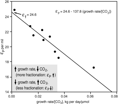
where all of the physiological effects are bundled into one numerically determined value, b. In laboratory experiments with cultures of Emiliania huxleyi and several species of diatom, b did indeed vary with growth rate, and it was actually the ratio of growth rate to CO2 concentration that yielded the best correlation with εP values: isotopic fractionation increases when CO2 in the environment increases and/or when growth rate decreases.
Relationship between photosynthetic isotope fractionation (εp), growth rate, and dissolved CO2 concentration in a laboratory culture of Emiliania huxleyi
In the broad surveys of algae and suspended organic matter collected from surface waters around the world, growth rate was difficult to measure, but the b factor was found to vary with phosphate concentrations in the surface water— presumably because phosphate is one of the main growth-limiting nutrients— and alkenone-based εP values were best correlated with the ratio of phosphate concentration to CO2. This raises the possibility that εP values might provide clues to changes in the amount of marine primary productivity over geologic time, which is almost as titillating—and as frustrating—as the possibility of obtaining information about past CO2 concentrations. Titillating, because the history of marine productivity and its relationship to atmospheric CO2 concentrations, ocean circulation, and climate remains elusive. Frustrating, because one needs to know CO2 levels before one can determine growth rates, and vice versa.
Kate Freeman and her students at Pennsylvania State University—most notably Mark Pagani, now with his own biogeochemistry laboratory at Yale— have been bravely attacking this double-headed beast from all angles. They have acquired εP records from alkenone and foram δ13C measurements in a wide range of ancient marine sediments. Using data from the many calibrations of CO2 versus εP, and employing a variety of techniques and oceanographic information to constrain ancient surface water phosphate concentrations and the related b factor, they have estimated dissolved and atmospheric CO2 concentrations all the way back to the early Eocene epoch.
For the Miocene epoch, 25 to 5 million years ago, Pagani and his colleagues analyzed sediment cores from open ocean sites where nutrients are consistently low and there are no cycles of upwelling or input from adjacent landmasses, so it was fairly safe to assume that average growth rates had not changed much, and they used actual measurements of surface water phosphate concentrations to approximate values for the b factor. In older sediments, things become more problematic. Alkenones are relatively rare in sediments from the Eocene and Oligocene epochs, and Pagani had to patch together data from a variety of diff erent ocean environments, with varying nutrient and current regimes. Here the similarity of the observed trends in alkenone εP values at the diff erent sites provides some evidence that they were primarily determined by changes in atmospheric CO2 concentration and not by changes in nutrient cycling and availability, which would surely have been diff erent at each site. Of course, the coccolithophores were changing and evolving during these long time periods, and the alkenone-producing organisms that predated Emiliania huxleyi or Gephyrocapsa oceanica may have changed in ways that affected other components of the b factor, such as the alga’s cell size or its preference for obtaining carbon from dissolved bicarbonate rather than CO2. Though there is no conclusive way of eliminating this possibility, Pagani and colleagues argue eff ectively that the observed trends in εP are unlikely to be the result of such evolution.
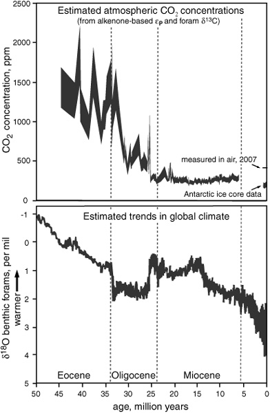
According to their provocative though still dubious reconstruction of atmospheric CO2 levels, climate and CO2 were not always as closely linked as they were during the past 100,000 years of ice age climates. A general, irreversible decline in atmospheric CO2 concentration during the Eocene and a dramatic drop at the beginning of the Oligocene period appear to be coupled to a steadily cooling climate, and may well have been responsible for it. But during the Miocene, atmospheric CO2 levels remained relatively low and unchanged, while the climate proxies attest to significant, irreversible changes in the global climate. This is in keeping with the hypothesis that major global climatic trends during this period were determined by tectonic plate movements and opening of the Drake Passage between South America and Antarctica, which initiated the circumpolar current that isolates Antarctica and led to formation of the East Antarctic ice sheet.
It is the beauty of the Ocean Drilling Program that Pagani and his colleagues have been able to extract such an amazing amount of information from what is, in essence, an ambiguous measurement. A more rigorous reconstruction of the history of atmospheric CO2 levels must await development of reliable independent proxies for growth rate or surface-water nutrient concentrations and, perhaps, more insight into the alkenone-producing organisms that predated Emily, or the calibration and use of εP values derived from δ13C values for other algal biomarkers, such as dinosterol and dinosterane or the HBIs. Richard Pancost, another of Freeman’s students, worked with her and Wakeham to explore such possibilities, measuring the δ13C of various diatom sterols and dinosterol in suspended organic matter from surface waters off the coast of Peru, where upwelling creates a gradient of dissolved CO2 and nutrient concentrations as one moves away from the coast. But their attempts to calibrate εP values determined for diatoms and dinoflagellates, with dissolved CO2 concentrations and growth rates approximated from nutrient concentrations, met with limited success. Diatom cell size and carbon transport mechanisms vary greatly among species and genera, and none of the diatom sterols were specific enough to provide a good proxy. And for reasons that are still unclear, the dinosterol δ13C values in the Peru samples were nearly constant, little influenced by either changing nutrient or CO2 concentrations. But even as biomarker paleo-CO2 and growth rate proxies await redemption or discovery, the ability to determine the isotopic composition of individual biomarkers has opened doors to understanding relationships between climate and ecology on many other fronts.
The history of CO2 and climate
As soon as Geoff saw that Hayes and his students had come up with a mass spectrometer that allowed one to determine the 13C content of specific compounds in a sediment extract, he found a British instrument company that had developed a prototype of a similar instrument and started trying it out on his leaf wax n-alkanes, using the δ13C values and chain-length distributions to distinguish among species of trees and track their inputs in lake sediments. The most useful application of such data to date, however, involves a much broader distinction among plant types than that among species or genera, or even families, a distinction that reflects fundamental biochemical diff erences in their photosynthetic pathways.
Like algae, most trees, shrubs, and northern grasses operate with what’s known as C3 photosynthesis, employing the Calvin cycle’s rubisco enzyme for the initial assimilation of CO2 into a 3-carbon sugar. But tropical grasses and some salt-marsh grasses use C4 photosynthesis, where the initial capture of CO2 is facilitated by an enzyme with a greater affinity for CO2 and a less discriminating taste in carbon isotopes than rubisco’s. In these plants, the CO2 is incorporated into a four-carbon acid and ferried into a special set of cells within the leaf, where it accumulates, isolated from the atmosphere. Here the Calvin cycle takes over and the finicky rubisco, now supplied with a high concentration of CO2 and protected from oxygen in the atmosphere, operates quite efficiently and with less isotope discrimination. These C4 plants are generally well adapted to drought and high temperatures, and on the contemporary earth they dominate the huge areas of arid grassland and savanna in subtropical Africa, South America, Australia, and South Asia. Their complicated system of photosynthesis apparently requires more energy to run than C3 photosynthesis, putting them at a disadvantage in cool, moist climates.
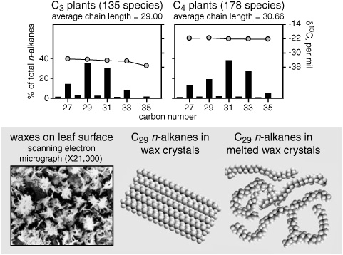
Geoff’s group’s initial compound-specific isotope investigations of n-alkanes in the leaf waxes of C4 plants revealed that their δ13C values were consistently 10–15 per mil less depleted in 13C than the corresponding compounds in C3 plants, reflecting the less finicky nature of the CO2-fixing enzyme in C4 plants. In what would appear to be a lifelong extension of the project he started in Tenerife in 1960, and true to the legacy of the Cambridge biochemist whose cigarette tins full of leaf waxes launched his career as a natural historian of molecules, Geoff has been working with Jürgen’s student Florian Rommerskirchen on a new collection of leaf waxes from African plants. With the isotope information added, the chain-length distributions are more distinct than they ever were in the Tenerife study. Surveys of the n-alkanes and n-alkanols in leaf waxes from hundreds of species of plants and grasses have confirmed that these compounds in C4 plants are consistently less 13C depleted, and their homologue distributions more skewed toward longer chain lengths, than they are in C3 plants. The n-alkanes in C4 plants have an average δ13C of about −22 per mil, as opposed to −34 per mil for C3 plants, and an average chain length of 31 carbon atoms, compared to 29 for the C3 n-alkanes. The isotopic difference between the two plant types clearly stems from their diff erent methods of assimilating carbon. The chain-length difference may be directly related to C4 plants’ competitive success in warm, arid climes. When skies are clear and the sun shines directly on a plant’s leaves, leaf surfaces can become so hot that the waxes melt and lose their protective qualities, including the ability to guard against drought. But the compounds with longer carbon chains have slightly higher melting points, and their relative abundance in C4 plants may be just enough to keep the molecules aligned in the wax crystals under these conditions.
C3 vs. C4 plants: n-alkane distributions and δ13C values
Unlike algae, which assimilate bicarbonate or CO2 directly from the water in their environment, the cells that fix carbon in land plants are protected within leaves, and CO2 collects in the leaves’ intercellular spaces before it is assimilated. The amount of CO2 available for assimilation is regulated to some extent by the opening and closing of pores in the leaf, so the direct eff ect of changes in atmospheric CO2 concentration on carbon isotope fractionation is less evident than it is in algae. Nevertheless, at very low atmospheric concentrations, C3 plants are hard-put to maintain the relatively high concentrations of CO2 that the rubisco enzyme needs to function efficiently, and C4 plants have a distinct advantage. Analyses of sediment cores from several mountain lakes in Kenya revealed that n-alkanes in sediments deposited during the last glacial period had relatively positive δ13C values and—taking into account the δ13C of atmospheric CO2 from the period, as measured in air trapped in the Greenland ice core—low fractionation factors, like those typical of C4 grasses. The onset of the interglacial period in this region was marked by a shift to the more pronounced fractionation and negative δ13C values typical of C3 plants. According to similar analyses of sediments from a lake in Guatemala, C4 plants also had the upper hand in Central America during the last glacial period. Given the C4 predilection for warm climes, this might seem counterintuitive. But conditions in these regions were not only cooler during glacial times, but considerably more arid, and the concentration of CO2 in the atmosphere was dramatically lower than during the interglacial period—enough, it seems, to have given the C4 plants a competitive edge. Sediments from a lake in northern Mexico, however, tell a diff erent story: in this region, C3 plants prevailed throughout the glacial period just as they do today, perhaps because extensive rainfall counterbalanced any advantage the C4 plants gained at low concentrations of CO2.
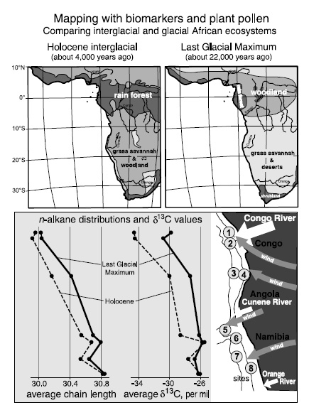
Paradoxically, some of the best information about regional changes in continental climate regimes and vegetation is coming not from lakes, but from marine sediments. Geoff has worked with Jürgen’s group and an interdisciplinary mix of northern German colleagues for years, analyzing Atlantic sediment cores from a north–south transect along the west coast of Africa in an attempt to map the changing ecosystems on the southern half of the continent during the last ice age cycle. They combined data from their analyses of isotopic compositions and distributions of leaf wax hydrocarbons in the sediments with a sharp-eyed Bremen palynologist’s counts of plant pollen grains and spores—blown out to sea with the dust, and taxonomically distinguished by their diff erent forms— and made use of geographers’ catalogues of vegetation types and atmospheric scientists’ calculations of wind trajectories to estimate the sources of dust at their study sites.
The ecosystems so determined for both the last glacial and the current interglacial periods reflect a general north–south trend from humid to arid conditions, with the average chain lengths of the n-alkanes and n-alkanols increasing and their δ13C values becoming less negative as one moves south from the equator and the ecosystems shift from C3 plant–dominated rain forest and woodlands to C4 plant–dominated grasslands and deserts. But at the height of the last glacial period, both the drier climes and the C4 grasslands clearly extended farther north into the equatorial region than they have during the Holocene interglacial.
Going back beyond the Holocene to a much earlier period of ice age cycles, the NIOZ scientists have studied the waxing and waning of C4 plant dominance in southern Africa between 1.2 million and 450,000 years ago. Focusing on a single long core from the Angola Basin, they chose the C31 n-alkane as an indicator, estimating the percentage of C4 plants from its δ13C values and the intensity of the trade winds and dust generation from its rate of accumulation in the sediments. Comparing these data with sea surface temperatures determined from alkenone values, and ice expansion and retreat from the foram δ18O values, they came to the conclusion that fluctuations in C4 plant prevalence for the region had been tied to the changing intensity of the monsoon system and degree of aridity, rather than to low CO2 concentrations during the ice ages.
Paleobotanists who attempt to reconstruct the evolution of ecosystems in a region from the fossil plant record are often unable to quantify the relative importance of diff erent groups of plants—they may well see some trees in the forest, but the forest itself eludes them. The fossil record of C4 plants is particularly skimpy, because most of them lack fossil-forming woody parts. Biomarker and pollen studies of lake and coastal marine sediments now off er some recourse, providing a view of changing ecosystem type over an entire watershed or wind source region. One thing that has become clear in these studies is that for a given level of atmospheric CO2, there is a climate optimum where C4 plants can compete efficiently with C3 plants and dominate an ecosystem—up to a certain point. Farquhar’s laboratory experiments with CO2 uptake indicate that even in an exceptionally dry, hot climate, if atmospheric CO2 were to rise above 500 ppm, it would be impossible for C4 grasses to compete with C3 plants.
The oldest fossil evidence of C4 plants is from the mid-Miocene, and there is some evidence from the fossil teeth of herbivores that C4 grasses thrived during the late Miocene period. According to the ice-core records and alkenone εP values, atmospheric CO2 concentrations have not exceeded 500 ppm during the past 25 million years. But Pagani’s somewhat more tentative estimates from earlier time periods suggest that it rose above this level during the Oligocene and was well above 1,000 ppm during the Eocene. The even cruder estimates for the Cretaceous period—based on models of the carbon cycle, ancient soils, εP values of porphyrins, and an array of marine algal biomarkers—vary widely but are all well above the 500 ppm limit, ranging from 900 ppm all the way up to 3,300 ppm. It would thus seem unlikely that C4 plants could have thrived much before the Miocene, and some theories of plant evolution hold that the C4 photosynthetic pathway in tropical grasses was, in part, an adaptation to decreasing atmospheric CO2 levels at this time. It may, however, have evolved repeatedly in diff erent types of plants before it found its contemporary home in the grasses, and there is some evidence that it was already in existence during the Cretaceous.
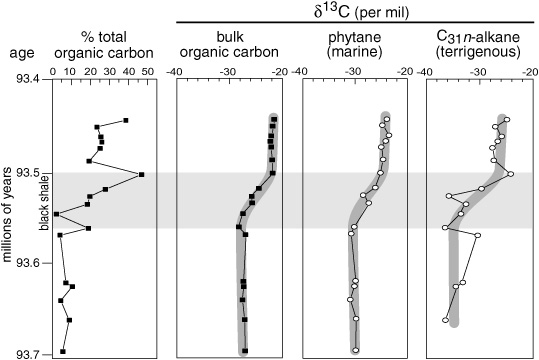
Multiproxy investigations of Cretaceous black shales indicate that CO2 levels may have dropped dramatically during the oceanic anoxic events, in which case C4 plants might have seized the opportunity for their moment in the sun, just as they apparently did during the ice ages. Given the global distribution of these shales and their high content of organic matter, a huge amount of organic carbon was buried in the sediments during these events—carbon that would otherwise have been recycled to CO2 in the surface water. Values of δ13C for both the marine organic matter and the carbonates formed from bicarbonate typically shifted to more positive values over the course of black shale deposition, as more and more organic matter was buried and 12C was partitioned into the sediments. Such a massive burial of organic matter over half a million years would, presumably, have resulted in CO2 being sucked out of the atmosphere and might have been responsible for occasional cooling trends in the midst of an otherwise warm Cretaceous period. Isotope fractionation factors determined for porphyrins, sulfur-bound phytane, and C27 and C28 steranes in black shales deposited during one of the most pronounced oceanic anoxic events, about 93.5 million years ago, all suggest that there was a marked decrease in atmospheric CO2 at this time—though precisely how much is a matter of some contention, with estimates varying across studies, from 20% to 80%. The NIOZ group found additional evidence in the δ13C values of leaf wax n-alkanes, which shifted over the course of shale deposition from values in the −30 to −38 range typical of C3 plants toward the more positive values typical of C4 plants. They estimated that the change from C3 to C4 plant ecosystems occurred within 60,000 years of the onset of organic-matter–rich sediment deposition and proposed that this was the time required for burial of enough carbon to reduce the atmospheric CO2 concentration below the 500 ppm mark and allow C4 plants to get the upper hand.
The extraordinary dark bands of sediment discovered by the Deep Sea Drilling Project in the 1970s are finally providing something more than molecules for the collectors. But the realization that a bit of productive exuberance in the surface waters might have pushed the deep waters of a slowly circulating ocean system over the edge into anoxia for more than 100,000 years at a stretch—or that a pronounced CO2-based greenhouse eff ect that had persisted for most of the long Cretaceous was interrupted by this event, and, incidentally, that C4 photosynthesis may have evolved in land plants more than 90 million years ago—is only the beginning. The real surprises are coming not from the biomarkers of land plants and algae, but from those of smaller, more unassuming and sometimes downright anonymous organisms, which, as we shall see, have finally attracted the attention of microbiologists.
Did Cretaceous oceanic anoxic events allow C4 land plants to become more prevalent? Evidence from a DSDP core off the coast of northwest Africa
As the investigations of the Messel shale demonstrated, addition of the isotopic dimension to the structural information in the molecular lexicon makes it easier to link fossil molecules to source organisms, and to diff erentiate among possible sources for the same compound. But perhaps most important for understanding the contributions of microorganisms to an ecosystem, the isotopic makeup of a biomarker can link it directly to a biochemical process. The prevalence of organisms that obtain their sustenance by diff erent means—C3 or C4 photosynthesis, respiration, fermentation, or one of the various energy- and carbon-harnessing processes that microorganisms have construed—can now be assessed and environmental conditions inferred, even when those organisms leave no other trace of their existence. Even, indeed, when they comprise organisms that have completely eluded detection—unknown, hitherto unimagined extinct and, miraculously undiscovered, extant species. Commercially built GC-irm-MS has joined the ranks of organic geochemists’ most coveted tools, and compound-specific isotope analysis has become a crucial component in their investigations. With such tools in hand, they have joined ranks with microbiologists and molecular biologists, and the rich, varied, microbial life of natural environments has thrown open its doors to exploration, yielding astonishing discoveries at every turn.