11
Contrasts
One of the hardest things about learning to do statistics is knowing how to interpret the output produced by the model that you have fitted to data. The reason why the output is hard to understand is that it is based on contrasts, and the idea of contrasts may be unfamiliar to you.
Contrasts are the essence of hypothesis testing and model simplification. They are used to compare means or groups of means with other means or groups of means, in what are known as single degree of freedom comparisons. There are two sorts of contrasts we might want to carry out:
- contrasts we had planned to carry out at the experimental design stage (these are referred to as a priori contrasts)
- contrasts that look interesting after we have seen the results (these are referred to as a posteriori contrasts)
Some people are very snooty about a posteriori contrasts, on the grounds that they were unplanned. You are not supposed to decide what comparisons to make after you have seen the analysis, but scientists do this all the time. The key point is that you should only do contrasts after the ANOVA has established that there really are significant differences to be investigated. It is bad practice to carry out tests to compare the largest mean with the smallest mean, if the ANOVA fails to reject the null hypothesis (tempting though this may be).
There are two important points to understand about contrasts:
- there is a huge number of possible contrasts
- there are only k − 1 orthogonal contrasts
where k is the number of factor levels. Two contrasts are said to be orthogonal to one another if the comparisons are statistically independent. Technically, two contrasts are orthogonal if the products of their contrast coefficients sum to zero (we shall see what this means in a moment).
Let's take a simple example. Suppose we have one factor with five levels and the factor levels are called a, b, c, d and e. Let us start writing down the possible contrasts. Obviously we could compare each mean singly with every other:

but we could also compare pairs of means:

or triplets of means:

or groups of four means:

I think you get the idea. There are absolutely masses of possible contrasts. In practice, however, we should only compare things once, either directly or implicitly. So the two contrasts a vs. b and a vs. c implicitly contrast b vs. c. This means that if we have carried out the two contrasts a vs. b and a vs. c then the third contrast b vs. c is not an orthogonal contrast because you have already carried it out, implicitly. Which particular contrasts are orthogonal depends very much on your choice of the first contrast to make. Suppose there were good reasons for comparing {a, b, c, e} vs. d. For example, d might be the placebo and the other four might be different kinds of drug treatment, so we make this our first contrast. Because k − 1 = 4 we only have three possible contrasts that are orthogonal to this. There may be a priori reasons to group {a, b} and {c, e}, so we make this our second orthogonal contrast. This means that we have no degrees of freedom in choosing the last two orthogonal contrasts: they have to be a vs. b and c vs. e. Just remember that with orthogonal contrasts you compare things only once.
Contrast Coefficients
Contrast coefficients are a numerical way of embodying the hypothesis we want to test. The rules for constructing contrast coefficients are straightforward:
- treatments to be lumped together get the same sign (plus or minus)
- groups of means to be contrasted get opposite sign
- factor levels to be excluded get a contrast coefficient of 0
- the contrast coefficients must add up to 0
Suppose that with our five-level factor  we want to begin by comparing the four levels {a, b, c, e} with the single level d. All levels enter the contrast, so none of the coefficients is 0. The four terms {a, b, c, e} are grouped together so they all get the same sign (minus, for example, although it makes no difference which sign is chosen). They are to be compared to d, so it gets the opposite sign (plus, in this case). The choice of what numeric values to give the contrast coefficients is entirely up to you. Most people use whole numbers rather than fractions, but it really doesn't matter. All that matters is that the values chosen sum to 0. The positive and negative coefficients have to add up to the same value. In our example, comparing four means with one mean, a natural choice of coefficients would be −1 for each of {a, b, c, e} and +4 for d. Alternatively, we could have selected +0.25 for each of {a, b, c, e} and −1 for d.
factor level: a b c d econtrast 1 coefficients, c: -1 -1 -1 4 -1
Suppose the second contrast is to compare {a, b} with {c, e}. Because this contrast excludes d, we set its contrast coefficient to 0. {a, b} get the same sign (say, plus) and {c, e} get the opposite sign. Because the number of levels on each side of the contrast is equal (two in both cases) we can use the same numeric value for all the coefficients. The value 1 is the most obvious choice (but you could use 13.7 if you wanted to be perverse):
factor level: a b c d econtrast 2 coefficients, c: 1 1 -1 0 -1
There are only two possibilities for the remaining orthogonal contrasts: a vs. b and c vs. e:
factor level: a b c d econtrast 3 coefficients, c: 1 -1 0 0 0contrast 4 coefficients, c: 0 0 1 0 -1
An Example of Contrasts in R
The example comes from the competition experiment we analysed in Chapter 9 in which the biomass of control plants is compared to the biomass of plants grown in conditions where competition was reduced in one of four different ways. There are two treatments in which the roots of neighbouring plants were cut (to 5 cm depth or 10 cm) and two treatments in which the shoots of neighbouring plants were clipped (25% or 50% of the neighbours cut back to ground level; see p. 162).
comp <- read.csv("c:\\temp\\competition.csv")attach(comp)names(comp)[1] "biomass" "clipping"
We start with the one-way ANOVA:
model1 <- aov(biomass~clipping)summary(model1)Df Sum Sq Mean Sq F value Pr(>F)clipping 4 85356 21339 4.302 0.00875 **Residuals 25 124020 4961
Clipping treatment has a highly significant effect on biomass. But have we fully understood the result of this experiment? I don't think so. For example, which factor levels had the biggest effect on biomass? Were all of the competition treatments significantly different from the controls ? To answer these questions, we need to use summary.lm:
summary.lm(model1)Coefficients:Estimate Std. Error t value Pr(>|t|)(Intercept) 465.17 28.75 16.177 9.4e-15 ***clippingn25 88.17 40.66 2.168 0.03987 *clippingn50 104.17 40.66 2.562 0.01683 *clippingr10 145.50 40.66 3.578 0.00145 **clippingr5 145.33 40.66 3.574 0.00147 **Residual standard error: 70.43 on 25 degrees of freedomMultiple R-squared: 0.4077, Adjusted R-squared: 0.3129F-statistic: 4.302 on 4 and 25 DF, p-value: 0.008752
It looks as if we need to keep all five parameters, because all five rows of the summary table have one or more significance stars. If fact, this is not the case. This example highlights the major shortcoming of treatment contrasts (the default contrast method in R): they do not show how many significant factor levels we need to retain in the minimal adequate model.
A Priori Contrasts
In this experiment, there are several planned comparisons we should like to make. The obvious place to start is by comparing the control plants that were exposed to the full rigours of competition, with all of the other treatments.
levels(clipping)[1] "control" "n25" "n50" "r10" "r5"
That is to say, we want to contrast the first level of clipping with the other four levels. The contrast coefficients, therefore, would be 4, −1, −1, −1, −1. The next planned comparison might contrast the shoot-pruned treatments (n25 and n50) with the root-pruned treatments (r10 and r5). Suitable contrast coefficients for this would be 0, 1, 1, −1, −1 (because we are ignoring the control in this contrast). A third contrast might compare the two depths of root-pruning; 0, 0, 0, 1, −1. The last orthogonal contrast would therefore have to compare the two intensities of shoot-pruning: 0, 1, −1, 0, 0. Because the clipping factor has five levels there are only 5 − 1 = 4 orthogonal contrasts.
R is outstandingly good at dealing with contrasts, and we can associate these four user-specified a priori contrasts with the categorical variable called clipping like this:
contrasts(clipping) <-cbind(c(4,-1,-1,-1,-1),c(0,1,1,-1,-1),c(0,0,0,1,-1),c(0,1,-1,0,0))
We can check that this has done what we wanted by typing
contrasts(clipping)[,1] [,2] [,3] [,4]control 4 0 0 0n25 -1 1 0 1n50 -1 1 0 -1r10 -1 -1 1 0r5 -1 -1 -1 0
which produces the matrix of contrast coefficients that we specified. Note that all the columns add to zero (i.e. each set of contrast coefficients is correctly specified). Note also that the products of any two of the columns sum to zero (this shows that all the contrasts are orthogonal, as intended): for example comparing contrasts 1 and 2 gives products 0 + (−1) + (−1) + 1 + 1 = 0.
Now we can refit the model and inspect the results of our specified contrasts, rather than the default treatment contrasts:
model2 <- aov(biomass~clipping)summary.lm(model2)Coefficients:Estimate Std. Error t value Pr (>|t|)(Intercept) 561.80000 12.85926 43.688 < 2e-16 ***clipping1 -24.15833 6.42963 -3.757 0.000921 ***clipping2 -24.62500 14.37708 -1.713 0.099128 .clipping3 0.08333 20.33227 0.004 0.996762clipping4 -8.00000 20.33227 -0.393 0.697313Residual standard error: 70.43 on 25 degrees of freedomMultiple R-squared: 0.4077, Adjusted R-squared: 0.3129F-statistic: 4.302 on 4 and 25 DF, p-value: 0.008752
Instead of requiring five parameters (as suggested by our initial treatment contrasts), this analysis shows that we need only two parameters: the overall mean (561.8) and the contrast between the controls and the four competition treatments (p = 0.000921). All the other contrasts are non-significant. Notice than the rows are labelled by the variable name clipping pasted to the contrast number (1 to 4).
Treatment Contrasts
We have seen how to specify our own customized contrasts (above) but we need to understand the default behaviour of R. This behaviour is called treatment contrasts and it is set like this:
options(contrasts=c("contr.treatment","contr.poly"))
The first argument, "contr.treatment", says we want to use treatment contrasts (rather than Helmert contrasts or sum contrasts), while the second, "contr.poly", sets the default method for comparing ordered factors (where the levels are semi-quantitative like ‘low’, ‘medium’ and ‘high’). We shall see what these unfamiliar terms mean in a moment. Because we had associated our explanatory variable clipping with a set of user-defined contrasts (above), we need to remove these to get back to the default treatment contrasts, like this:
contrasts(clipping) <- NULL
Now let us refit the model and work out exactly what the summary is showing:
model3 <- lm(biomass~clipping)summary(model3)Coefficients:Estimate Std. Error t value Pr(>|t|)(Intercept) 465.17 28.75 16.177 9.4e-15 ***clippingn25 88.17 40.66 2.168 0.03987 *clippingn50 104.17 40.66 2.562 0.01683 *clippingr10 145.50 40.66 3.578 0.00145 **clippingr5 145.33 40.66 3.574 0.00147 **Residual standard error: 70.43 on 25 degrees of freedomMultiple R-squared: 0.4077, Adjusted R-squared: 0.3129F-statistic: 4.302 on 4 and 25 DF, p-value: 0.008752
First things first. There are five rows in the summary table, labelled (Intercept), clippingn25, clippingn50, clippingr10 and clippingr55. Why are there five rows? There are five rows in the summary table because this model has estimated five parameters from the data (one for each factor level). This is a very important point. Different models will produce summary tables with different numbers of rows. You should always be aware of how many parameters your model is estimating from the data, so you should never be taken by surprise by the number of rows in the summary table.
Next we need to think what the individual rows are telling us. Let us work out the overall mean value of biomass, to see if that appears anywhere in the table:
mean(biomass)[1] 561.8
No. I can't see that number anywhere. What about the five treatment means? We obtain these with the extremely useful tapply function:
tapply(biomass,clipping, mean)control n25 n50 r10 r5465.1667 553.3333 569.3333 610.6667 610.5000
This is interesting. The first treatment mean (465.1667 for the controls) does appear (in row number 1), but none of the other means are shown. So what does the value of 88.17 in row number 2 of the table mean? Inspection of the individual treatment means lets you see that 88.17 is the difference between the mean biomass for n25 and the mean biomass for the control. What about 104.17 ? That turns out to be the difference between the mean biomass for n50 and the mean biomass for the control. Treatment contrasts are expressed as the difference between the mean for a particular factor level and the mean for the factor level that comes first in the alphabet. No wonder they are hard to understand on first encounter.
Why does it all have to be so complicated? What's wrong with just showing the five mean values? The answer has to do with parsimony and model simplification. We want to know whether the differences between the means that we observe (e.g. using tapply) are statistically significant. To assess this, we need to know the difference between the means and (crucially) the standard error of the difference between two means (see p. 91 for a refresher on this). The summary.lm table is designed to make this process as simple as possible. It does this by showing us just one mean (the intercept) and all the other rows are differences between means. Likewise, in the second column, it shows us just one standard error (the standard error of the mean for the intercept – the control treatment in this example), and all of the other values are the standard error of the difference between two means. So the value in the top row (28.75) is much smaller than the values in the other four rows (40.66) because the standard error of a mean is

while the standard error of the difference between two means is
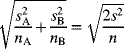
You can see that for the simplest case where (as here) we have equal replication in all five factor levels (n = 6) and we intend to use the pooled error variance s2, the standard error of the difference between two means is  times the size of the standard error of a mean. Let us check this out for our example
28.75*sqrt(2)[1] 40.65864
So that checks out. What if it is not convenient to compare the means with the factor level that happens to come first in the alphabet ? Then all we need to do is change the order of the levels with a new factor declaration, in which we specify the order in which the factor levels are to be considered. You can see an example of this on p. 242. Alternatively, you can define the contrasts attributes of the factor, as we saw earlier in this chapter.
Model Simplification by Stepwise Deletion
Model simplification with treatment contrasts requires that we aggregate non-significant factor levels in a stepwise a posteriori procedure. The results we get by doing this are exactly the same as those obtained by defining the contrast attributes of the explanatory variable as we did earlier.
Looking down the list of parameter estimates, we see that the most similar effect sizes are for r5 and r10 (the effects of root pruning to 5 and 10 cm): 145.33 and 145.5, respectively. We shall begin by simplifying these to a single root-pruning treatment called root. The trick is to use ‘levels gets’ to change the names of the appropriate factor levels. Start by copying the original factor name:
clip2 <- clipping
Now inspect the level numbers of the various factor level names:
levels(clip2)[1] "control" "n25" "n50" "r10" "r5"
The plan is to lump together r10 and r5 under the same name, ‘root’. These are the fourth and fifth levels of clip2 (count them from the left), so we write:
levels(clip2)[4:5] <- "root"
and to see what has happened we type:
levels(clip2)[1] "control" "n25" "n50" "root"
We see that "r10" and "r5" have been merged and replaced by "root". The next step is to fit a new model with clip2 in place of clipping, and to use anova to test whether the new simpler model with only four factor levels is significantly worse as a description of the data:
model4 <- lm(biomass~clip2)anova(model3,model4)Analysis of Variance TableModel 1: biomass ~ clippingModel 2: biomass ~ clip2Res.Df RSS Df Sum of Sq F Pr(>F)1 25 1240202 26 124020 -1 -0.0833333 0.0000168 0.9968
As we expected, this model simplification was completely justified. The next step is to investigate the effects using summary:
summary(model4)Coefficients:Estimate Std. Error t value Pr(>|t|)(Intercept) 465.17 28.20 16.498 2.72e-15 ***clip2n25 88.17 39.87 2.211 0.036029 *clip2n50 104.17 39.87 2.612 0.014744 *clip2root 145.42 34.53 4.211 0.000269 ***Residual standard error: 69.07 on 26 degrees of freedomMultiple R-squared: 0.4077, Adjusted R-squared: 0.3393F-statistic: 5.965 on 3 and 26 DF, p-value: 0.003099
Next, we want to compare the two shoot-pruning treatments with their effect sizes of 88.17 and 104.17. They differ by 16.0 (much more than the root-pruning treatments did), but you will notice that the standard error of the difference if 39.87. You will soon get used to doing t tests in your head and using the rule of thumb that t needs to be bigger than 2 for significance. In this case, the difference would need to be at least 2 × 39.87 = 79.74 for significance, so we predict that merging the two shoot pruning treatments will not cause a significant reduction in the explanatory power of the model. We can lump these together into a single shoot-pruning treatment as follows:
clip3 <- clip2levels(clip3)[2:3] <- "shoot"levels(clip3)[1] "control" "shoot" "root"
Then we fit a new model with clip3 in place of clip2:
model5 <- lm(biomass~clip3)anova(model4,model5)Analysis of Variance TableModel 1: biomass ~ clip2Model 2: biomass ~ clip3Res.Df RSS Df Sum of Sq F Pr(>F)1 26 1240202 27 124788 -1 -768 0.161 0.6915
Again, this simplification was fully justified. Do the root and shoot competition treatments differ?
summary(model5)Coefficients:Estimate Std. Error t value Pr(>|t|)(Intercept) 465.17 27.75 16.760 8.52e-16 ***clip3shoot 96.17 33.99 2.829 0.008697 **clip3root 145.42 33.99 4.278 0.000211 ***Residual standard error: 67.98 on 27 degrees of freedomMultiple R-squared: 0.404, Adjusted R-squared: 0.3599F-statistic: 9.151 on 2 and 27 DF, p-value: 0.0009243
The two effect sizes differ by 145.42 − 96.17 = 49.25 with a standard error of 33.99 (giving t < 2) so we shall be surprised if merging the two factor levels causes a significant reduction in the model's explanatory power:
clip4 <- clip3levels(clip4)[2:3] <- "pruned"levels(clip4)[1] "control" "pruned"
Now we fit a new model with clip4 in place of clip3:
model6 <- lm(biomass~clip4)anova(model5,model6)Analysis of Variance TableModel 1: biomass ~ clip3Model 2: biomass ~ clip4Res.Df RSS Df Sum of Sq F Pr(>F)1 27 1247882 28 139342 -1 -14553 3.1489 0.08726 .
This simplification was close to significant, but we are ruthless (p > 0.05), so we accept the simplification. Now we have the minimal adequate model:
summary(model6)Coefficients:Estimate Std. Error t value Pr (>|t|)(Intercept) 465.2 28.8 16.152 1.01e-15 ***clip4pruned 120.8 32.2 3.751 0.000815 ***Residual standard error: 70.54 on 28 degrees of freedomMultiple R-squared: 0.3345, Adjusted R-squared: 0.3107F-statistic: 14.07 on 1 and 28 DF, p-value: 0.0008149
It has just two parameters: the mean for the controls (465.2) and the difference between the control mean and the four other treatment means (465.2 + 120.8 = 586.0):
tapply(biomass,clip4,mean)control pruned465.1667 585.9583
We know from the p value = 0.000815 (above) that these two means are significantly different, but just to show how it is done, we can make a final model7 that has no explanatory variable at all (it fits only the overall mean). This is achieved by writing y~1 in the model formula (parameter 1, you will recall, is the intercept in R):
model7 <- lm(biomass~1)anova(model6,model7)Analysis of Variance TableModel 1: biomass ~ clip4Model 2: biomass ~ 1Res.Df RSS Df Sum of Sq F Pr(>F)1 28 1393422 29 209377 -1 -70035 14.073 0.0008149 ***
Note that the p value is exactly the same as in model6. The p values in R are calculated such that they avoid the need for this final step in model simplification: they are ‘p on deletion’ values.
It is informative to compare what we have just done by stepwise factor-level reduction with what we did earlier by specifying the contrast attribute of the factor.
Contrast Sums of Squares by Hand
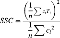
The key point to understand is that the treatment sum of squares SSA is the sum of all k − 1 orthogonal sums of squares. It is very useful to know which of the contrasts contributes most to SSA, and to work this out, we compute a set of contrast sums of squares SSC as follows:
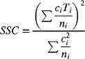
or, when all the sample sizes are the same for each factor level:
The significance of a contrast is judged in the usual way by carrying out an F test to compare the contrast variance with the pooled error variance,  from the ANOVA table. Since all contrasts have a single degree of freedom, the contrast variance is equal to SSC, so the F test is just

The contrast is significant (i.e. the two contrasted groups have significantly different means) if the calculated value of the test statistic is larger than the critical value of F with 1 and k(n − 1) degrees of freedom. We demonstrate these ideas by continuing our example. When we did factor-level reduction in the previous section, we obtained the following sums of squares for the four orthogonal contrasts that we carried out (the figures come from the model-comparison ANOVA tables, above):
| Contrast | Sum of squares |
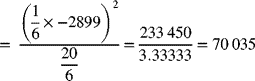
| Control vs. the rest | 70 035 |
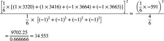
| Shoot pruning vs. root pruning | 14 553 |
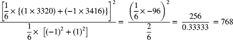
| Intense vs. light shoot pruning | 768 |
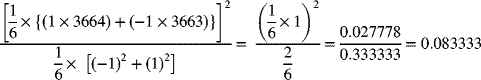
| Deep vs. shallow root pruning | 0.083 |
| Total |
What we shall do now is carry out the calculations involved in the a priori contrasts in order to demonstrate that the results are identical. The new quantities we need to compute the contrast sums of squares SSC are the treatment totals,  , in the formula above and the contrast coefficients
  . It is worth writing down the contrast coefficients again (see p. 214, above):
| Contrast | Contrast coefficients |
| Control vs. the rest |  |
| Shoot pruning vs. root pruning |  |
| Intense vs. light shoot pruning |  |
| Deep vs. shallow root pruning |  |
We use tapply to obtain the five treatment totals:
tapply(biomass,clipping,sum)control n25 n50 r10 r52791 3320 3416 3664 3663
For the first contrast, the contrast coefficients are 4, −1, −1, −1, and −1. The formula for SSC is therefore
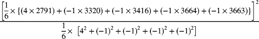
In the second contrast, the coefficient for the control is zero, so we leave this out:
The third contrast ignores the root treatments, so:
Finally, we compare the two root pruning treatments:
You will see that these sums of squares are exactly the same as we obtained by stepwise factor-level reduction. So don't let anyone tell you that these procedures are different or that one of them is superior to the other.
The Three Kinds of Contrasts Compared
You are very unlikely to need to use Helmert contrasts or sum contrasts in your work, but if you need to find out about them, they are explained in detail in The R Book (Crawley, 2013).
Reference
- Crawley, M.J. (2013) The R Book, 2nd edn, John Wiley & Sons, Chichester.
Further Reading
- Ellis, P.D. (2010) The Essential Guide to Effect Sizes: Statistical Power, Meta-Analysis, and the Interpretation of Research Results, Cambridge University Press, Cambridge.
- Miller, R.G. (1997) Beyond ANOVA: Basics of Applied Statistics, Chapman & Hall, London.