16
Death and Failure Data

Time-to-death data, and data on failure times, are often encountered in statistical modelling. The main problem is that the variance in such data is almost always non-constant, and so standard methods are inappropriate. If the errors are gamma distributed, then the variance is proportional to the square of the mean (recall that with Poisson errors, the variance is equal to the mean). It is straightforward to deal with such data using a generalized linear model (GLM) with gamma errors.

This case study has 50 replicates in each of three treatments: an untreated control, low dosage and high dosage of a novel cancer treatment. The response is the age at death for the rats (expressed as an integer number of months):

mortality <- read.csv("c:\\temp\\deaths.csv")
attach(mortality)
names(mortality)
[1] "death"     "treatment"    
tapply(death,treatment,mean)
	control   	 high   	  low 
	3.46   	 6.88   	 4.70

The animals receiving the high dose lived roughly twice as long as the untreated controls. The low dose increased life expectancy by more than 35%. The variance in age at death, however, is not constant:

tapply(death,treatment,var)
	  control  	    high	       low 
0.4167347 	2.4751020 	0.8265306

The variance is much greater for the longer-lived individuals, so we should not use standard statistical models which assume constant variance and normal errors. But we can use a GLM with gamma errors:

model <- glm(death~treatment,Gamma)
summary(model)
Coefficients:

	               	Estimate 	Std. Error 	t value 	Pr(>|t|) 
(Intercept)   	 0.289017   	0.008327  	34.708  	< 2e-16 ***
treatmenthigh 	-0.143669 	  0.009321 	-15.414 	 < 2e-16 ***
treatmentlow  	-0.076251 	  0.010340  	-7.374 	1.11e-11 ***
(Dispersion parameter for Gamma family taken to be 0.04150576)
          Null deviance: 17.7190  on 149  degrees of freedom
Residual deviance:  5.8337  on 147  degrees of freedom
AIC: 413.52
Number of Fisher Scoring iterations: 4

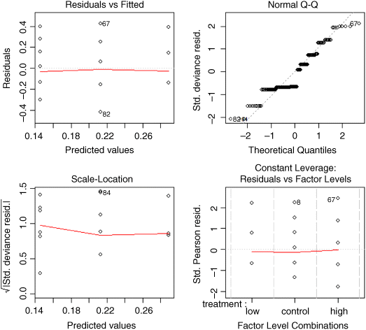
The link function with gamma errors is the reciprocal: that is why the parameter for the high dose appears as a negative term in the summary table: the mean value for high dose is calculated as 0.289 − 0.1437 = 0.1453, and 1/0.1453 = 6.882. Checking the model using plot(model) shows that it is reasonably well behaved (you might like to compare the behaviour of lm(death~treatment)). We conclude that all three treatment levels are significantly different from one another.

A common difficulty with data on time at death is that some (or even many) of the individuals do not die during the trial, so their age at death remains unknown (they might recover, they might leave the trial, or the experiment might end before they die). These individuals are said to be censored. Censoring makes the analysis much more complicated, because the censored individuals provide some information (we know the age at which they were last seen alive) but the data are of a different type from the information on age at death which is the response variable in the main analysis. There is a whole field of statistical modelling for such data: it is called survival analysis.

detach(mortality)

Survival Analysis with Censoring

The next example comes from a study of mortality in 150 wild male sheep. There were three experimental groups, and the animals were followed for 50 months. The groups were treated with three different medicines against their gut parasites: group A received a bolus with a high dose of worm-killer, group B received a low dose, and group C received the placebo (a bolus with no worm-killing contents). The initial body mass of each individual (weight) was recorded as a covariate. The month in which each animal died (death) was recorded, and animals which survived up to the 50th month (the end of the study) were recorded as being censored (they thus have censoring indicator status = 0, whereas the animals that died all have status = 1).

library(survival)
sheep <- read.csv("c:\\temp\\sheep.deaths.csv")
attach(sheep)
names(sheep)
[1] "death"  "status" "weight" "group"

The overall survivorship curves for the three groups of animals are obtained like this:

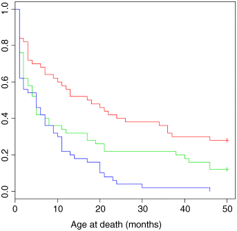
plot(survfit(Surv(death,status)~group),col=c(2,3,4),
                                                                                          xlab="Age at death (months)")

The crosses + at the end of the survivorship curves for groups A (red) and B (green) indicate that there was censoring in these groups (not all of the individuals were dead at the end of the experiment). Parametric regression in survival models uses the survreg function, for which you can specify a wide range of different error distributions. Here we use the exponential distribution for the purposes of demonstration (you can chose from dist = "extreme", "logistic", "gaussian" or "exponential" and from link = "log" or "identity"). We fit the full analysis of covariance model to begin with:

model <- survreg(Surv(death,status)~weight*group,dist="exponential")
summary(model)
Call:
survreg(formula = Surv(death, status) ~ weight * group, dist = "exponential")
                		Value 	Std. Error    	  z   	     p
(Intercept)    	3.8702   	  0.3854 	10.041 	1.00e-23
weight      	  -0.0803   	  0.0659	 -1.219 	2.23e-01
groupB   	     -0.8853 	    0.4508 	-1.964	 4.95e-02
groupC     	   -1.7804 	    0.4386 	-4.059	 4.92e-05
weight:groupB 	 0.0643    	 0.0674 	 0.954	 3.40e-01
weight:groupC 	 0.0796   	  0.0674 	 1.180	 2.38e-01
Scale fixed at 1 
Exponential distribution
Loglik(model)= -480.6   Loglik(intercept only)= -502.1
                    Chisq= 43.11 on 5 degrees of freedom, p= 3.5e-08 
Number of Newton-Raphson Iterations: 5 
n= 150

Model simplification proceeds in the normal way. You could use update, but here (for variety only) we refit progressively simpler models and test them using anova. First we take out the different slopes for each group:

model2 <- survreg(Surv(death,status)~weight+group,dist="exponential")
anova(model,model2,test="Chi")
   Terms Resid. Df  -2*LL       Test Df  Deviance P(>|Chi|)
1  weight * group     144 961.1800                NA         NA        NA
2  weight + group     146 962.9411  -weight:group -2  -1.761142 0.4145462

The interaction is not significant so we leave it out and try deleting weight:

model3 <- survreg(Surv(death,status)~group,dist="exponential")
anova(model2,model3,test="Chi")
                          Terms Resid. Df        -2*LL         Test Df           Deviance            P(>|Chi|)
1     weight + group        146 962.9411                      NA                         NA                        NA
2                            group        147 963.9393     -weight -1     -0.9981333      0.3177626

This is not significant, so we leave it out and try deleting group:

model4 <- survreg(Surv(death,status)~1,dist="exponential")
anova(model3,model4,test="Chi")
          Terms Resid. Df                  -2*LL        Test Df          Deviance                   P(>|Chi|)
1          group            147            963.9393                   NA                            NA                                   NA
2                    1          149         1004.2865              -2         -40.34721        1.732661e-09

This is highly significant, so we add it back. The minimal adequate model is model3 with the three-level factor group, but there is no evidence that initial body weight had any influence on survival.

summary(model3)
Call:
survreg(formula = Surv(death, status) ~ group, dist = "exponential")
            	 Value 	Std. Error   	 z	p
(Intercept) 	 3.467   	   0.167 	20.80 	3.91e-96
groupB     	 -0.671  	    0.225	 -2.99	 2.83e-03
groupC     	 -1.386   	   0.219 	-6.34 	2.32e-10
Scale fixed at 1 
Exponential distribution
Loglik(model)= -482   Loglik(intercept only)= -502.1
                    Chisq= 40.35 on 2 degrees of freedom, p= 1.7e-09 
Number of Newton-Raphson Iterations: 5 
n= 150

We need to retain all three groups (group B is significantly different from both group A and group C).

It is straightforward to compare error distributions for the same model structure:

model3 <- survreg(Surv(death,status)~group,dist="exponential")
model4 <- survreg(Surv(death,status)~group,dist="extreme")
model5 <- survreg(Surv(death,status)~group,dist="gaussian")
model6 <- survreg(Surv(death,status)~group,dist="logistic")
anova(model3,model4,model5,model6)
  Terms Resid. Df     -2*LL Test Df    Deviance Pr(>Chi)
1 group       147  963.9393     NA                      NA       NA
2 group       146 1225.3512     =    1 -261.411949       NA
3 group       146 1178.6582     =    0   46.692975       NA
4 group       146 1173.9478     =    0    4.710457       NA

Our initial choice of exponential was clearly the best, giving much the lowest residual deviance (963.94).

You can immediately see the advantage of doing proper survival analysis when you compare the predicted mean ages at death from model3 with the crude arithmetic averages of the raw data on age at death:

tapply(predict(model3,type="response"),group,mean)
        A    	    B   	 C 
 32.05555 	16.38635	 8.02
tapply(death,group,mean)
    A   	  B  	   C 
23.08 	14.42 	 8.02

If there is no censoring (as in group C, where all the individuals died) then the estimated mean ages at death are identical. But when there is censoring, the arithmetic mean underestimates the age at death, and when the censoring is substantial (as in group A) this underestimate is very large (23.08 vs. 32.06 months).

Survival Analysis with Censoring

Further Reading