Case study–Python for one-way ANOVA
A team member wants to compare the viscosity of four epoxy resins. She collects viscosity data from the four resins. She then performs one-way ANOVA to test for the equality of viscosity means of the four resins, using the model from StatsModels and then using a model from SciPy. Because the p values generated from both models are smaller than 0.05, she rejects the null hypothesis and concludes that there is a difference between viscosity means of the four resins.
One-way ANOVA is applied to test whether the levels of a factor on a one-way layout are different from each other. This one-way layout of a single factor consists of several levels and multiple data points at each level.
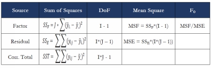
The following table summarizes the mathematical formula for one-way ANOVA
analysis:
[20]
Where:

= the jth data value from level i
I = the number of levels
J = the number of observations
DoF = the degree of freedom
One-way ANOVA using a model from StatsModels follows following steps.
Step 1. Import libraries.
In [1]:
import statsmodels.api as sm
from statsmodels.formula.api import ols
import pandas as pd
from scipy import stats
The statsmodels provides classes and functions for statistical analysis. Its ols is an ordinary least squares model.
Step 2. Load and examine the dataset.
In [2]:
df = pd.read_excel('case one way anova.xlsx')
In [3]:
print(df)
Resin Viscosity
0 1 922.2
1 1 742.4
2 1 539.4
3 1 1055.6
4 1 870.0
5 1 614.8
6 1 1049.8
7 1 870.0
8 1 667.0
9 1 1183.2
10 1 997.6
11 1 742.4
12 2 800.4
13 2 121.8
14 2 46.4
15 2 359.6
16 2 493.0
17 2 777.2
18 2 928.0
19 2 249.4
20 2 174.0
21 2 487.2
22 2 620.6
23 2 904.8
24 3 690.2
25 3 887.4
26 3 707.6
27 3 313.2
28 3 626.4
29 3 910.6
30 3 817.8
31 3 1015.0
32 3 835.2
33 3 440.8
34 3 754.0
35 3 1038.2
36 4 806.2
37 4 968.6
38 4 1264.4
39 4 945.4
40 4 916.4
41 4 1003.4
42 4 933.8
43 4 1096.2
44 4 1392.0
45 4 1073.0
46 4 1044.0
47 4 1131.
0
In [4]:
df.info()
<class 'pandas.core.frame.DataFrame'>
RangeIndex: 48 entries, 0 to 47
Data columns (total 2 columns):
Resin 48 non-null int64
Viscosity 48 non-null float64
dtypes: float64(1), int64(1)
memory usage: 848.0 bytes
The dataset has two columns, and each of them has 48 data points. The data in the first column indicates that there are four resins while the data in the second column are viscosity values. Notice that the data in the first column is categorical, although it is labeled as int64 by the DataFrame.info( ) function.
Step 3. Perform ordinary least squares analysis and fit the model.
In [5]:
moore_lm = ols('Viscosity ~ C(Resin, Sum)', data=df).fit()
The StatsModels’
ols( ) function performs an ordinary least squares regression, and its fit( ) function fits the model.
Step 4. Perform ANOVA analysi
s
In [6]:
table = sm.stats.anova_lm(moore_lm, typ=1)
In [7]:
print(table)
The sm.stats.anoma_1m( ) function generates an ANOVA table for one or more fitted linear models. The p-value (0.000007) is smaller than 0.05, leading to the rejection of the null hypothesis and the conclusion that there is a difference between the
viscosity means of the four resins.
One-way ANOVA using a model from SciPy follows the following steps.
Step 1. Set the Resin column as the index column.
In [8]:
df.set_index(['Resin'])
Out[8]:
|
Viscosity
|
|
Resin
|
|
|
1
|
922.2
|
|
1
|
742.4
|
|
1
|
539.4
|
|
1
|
1055.6
|
|
1
|
870.0
|
|
1
|
614.8
|
|
1
|
1049.8
|
|
1
|
870.0
|
|
1
|
667.0
|
|
1
|
1183.2
|
|
1
|
997.6
|
|
1
|
742.4
|
|
2
|
800.4
|
|
2
|
121.8
|
|
2
|
46.4
|
|
2
|
359.6
|
|
2
|
493.0
|
|
2
|
777.2
|
|
2
|
928.0
|
|
2
|
249.4
|
|
2
|
174.0
|
|
2
|
487.2
|
|
2
|
620.6
|
|
2
|
904.8
|
|
3
|
690.2
|
|
3
|
887.4
|
|
3
|
707.6
|
|
3
|
313.2
|
|
3
|
626.4
|
|
3
|
910.6
|
|
3
|
817.8
|
|
3
|
1015.0
|
|
3
|
835.2
|
|
3
|
440.8
|
|
3
|
754.0
|
|
3
|
1038.2
|
|
4
|
806.2
|
|
4
|
968.6
|
|
4
|
1264.4
|
|
4
|
945.4
|
|
4
|
916.4
|
|
4
|
1003.4
|
|
4
|
933.8
|
|
4
|
1096.2
|
|
4
|
1392.0
|
|
4
|
1073.0
|
|
4
|
1044.0
|
|
4
|
1131.
0
|
The DataFrame.set_index( ) function sets a list, a series, or a Data Frame as index of a Data Frame.
Step 2. Slice the Data Frame into four part, each for one resin.
In [9]:
x = df.loc[0:11]
print(x)
Resin Viscosity
0 1 922.2
1 1 742.4
2 1 539.4
3 1 1055.6
4 1 870.0
5 1 614.8
6 1 1049.8
7 1 870.0
8 1 667.0
9 1 1183.2
10 1 997.6
11 1 742.
4
In [10]:
y = df.loc[12:23]
print(y)
Resin Viscosity
12 2 800.4
13 2 121.8
14 2 46.4
15 2 359.6
16 2 493.0
17 2 777.2
18 2 928.0
19 2 249.4
20 2 174.0
21 2 487.2
22 2 620.6
23 2 904.8
In [11]:
z = df.loc[24:35]
print(z)
Resin Viscosity
24 3 690.2
25 3 887.4
26 3 707.6
27 3 313.2
28 3 626.4
29 3 910.6
30 3 817.8
31 3 1015.0
32 3 835.2
33 3 440.8
34 3 754.0
35 3 1038.
2
In [12]:
w=df.loc[36:47]
print(w)
Resin Viscosity
36 4 806.2
37 4 968.6
38 4 1264.4
39 4 945.4
40 4 916.4
41 4 1003.4
42 4 933.8
43 4 1096.2
44 4 1392.0
45 4 1073.0
46 4 1044.0
47 4 1131.0
The df.loc( ) function accesses a group of rows and columns by label(s) or a boolean array. In this case, the Data Frame is divided into four segments (x, y, z, and w), one segment for each of the four resins.
Step 3. Perform ANOVA analysis.
In [13]:
stats.f_oneway(x['Viscosity'], y['Viscosity'], z['Viscosity'], w['Viscosity'])
Out[13]:
F_onewayResult(statistic=12.112191467357228, pvalue=6.569949143423387e-06)
The SciPy’s stats.f_oneway( ) function performs an one-way ANOVA. Its returns have two values. The first one is the computed F-value of
the test, and the second one is the associated p-value from the F-distribution. Again, the null hypothesis is rejected because the p-value (6.57e-06) is much smaller than 0.05.