7
Measuring the Steepness of Flowing Paths

7.1. Summary of the chapter

As explained in the previous chapter, unweighted gravitational digraphs convey rich topographic information. However, in the absence of weights, all directed paths connecting a particular node with a black hole are, aside from their length, equivalent. This chapter proposes an order relation between the directed paths having a common origin, expressing the steepness of these paths. For this, we have to reintroduce node weights.

If the digraph is derived from the node-weighted graph G(ν, nil), we simply keep the node weights and replace each flowing edge with an arc, obtaining the digraph .

An edge-weighted graph G(nil, η) is first transformed into a flowing graph ↓ G(nil, η) by skipping the edges which are not the lowest edges of one of their extremities. This new graph has the same flowing edges whether we consider the initial edge weights or the node weights defined by ε_neη. Hence, we consider the node-weighted digraph for comparing the steepness of the directed paths.

The steepness of a directed path linking a node p with a node s belonging to a black hole will be characterized by considering the weights of the series of nodes belonging to the path, starting with the weight of p. The weight of the last node s is infinitely duplicated, yielding an infinite series of weights.

A lexicographic order relation is defined on infinite lists of weights. Between two directed paths with the same origin, the steepest is the one whose list of weights is the smallest for this lexicographic order relation.

Each node is the origin of one or several directed paths. At least one of them has a minimal lexicographic weight. Such paths with a minimal lexicographic weight are said to be ∞ – steep.

If another path has the same weights as the ∞ – steep path on its k first nodes, it is said to be k – steep. A digraph in which all directed paths are k – steep is said to be k – steep for k ≤ ∞.

7.2. Why do the catchment zones overlap?

7.2.1. Relation between the catchment zones and the flowing paths

We have chosen to study the topography of an edge- or node-weighted graph from a hydrographic point of view. The topographical structure of a graph entirely derives from definition of the flowing edges: a drop of water glides from node to node following the flowing edges. Flowing paths are all paths along which a drop of water may glide. The catchment zone of a regional minimum is the set of nodes linked to this minimum by a flowing path.

The deep similarities between the topography of node- and edge-weighted graphs appear as it is possible to associate with each of them a weightless gravitational digraph, on which the flowing paths become directed paths, the regional minima become black holes, each node belonging to the catchment zone of one or several black holes.

If a node is linked with two distinct black holes by two flowing paths, it belongs to both their catchment zones which overlap. If each node were linked with only one black hole through a flowing path, the catchment zones would not overlap but form a partition of catchment basins.

The overlapping of catchment zones is thus inherent in the graph structure. Reducing the number of directed paths linking a node with a black hole will reduce the catchment zone of this black hole.

7.2.2. Comparing the steepness of flowing paths

When we studied weighted graphs, we chose the most comprehensive definition of a flowing edge, simply forbidding that a drop of water moves upwards but allowing all other motions. As a result, the catchment zones are also the largest possible.

Every time a flowing path links a given node p with a black hole m, is cut, the node p ceases to belong to the catchment zone of m. We call the operation which cuts the first edges or arcs of flowing paths pruning. This pruning reduces the extension of the catchment zones and of their overlapping. Pruning should leave at least one flowing path connecting each node with a black hole; thus, each node still belongs to a catchment zone, and as often as possible, to only one catchment zone.

Of course, by skipping the node or edge weights, we are unable to discriminate between two flowing paths. In order to discriminate between the flowing paths which should be kept and those which may be suppressed, we have to reintroduce node or edge weights. Using these weights, it will be possible to order the flowing paths according to their steepness and prune those which are less steep. Suppressing flowing paths which are less steep and keeping the steeper ones will reduce the overlapping zones of the catchment basins. Two paths linking a node p with two distinct black holes may then be compared via a lexicographic order relation between their lists of weights; if the first edge of one of them is cut, then the node p will belong to only one catchment basin.

7.2.3. The redundancy between node and edge weights

If weights have to be reintroduced into a weightless gravitational digraph derived from a node- or edge-weighted flowing graph, should we reintroduce node weights or edge weights? We now recall how weights may be assigned to node-weighted graphs and node weights to edge-weighted graphs:

• – G(ν, nil): each edge is a flowing edge for one of its extremities and gets the same weight as this extremity. If the node weights are ν, the edge weights are δ_enν. In a flowing path of G(ν, δ_enν), each node is followed by an edge with the same weight except the ultimate node, when this node is an isolated black hole. Each flowing edge of G(ν, nil) is replaced by an arrow in the digraph (nil, nil).
• – G(nil, η): the edges that are not the lowest edges of one of their extremities are cut, producing ↓ G(nil, η). Each edge of ↓ G(nil, η) is then a flowing edge of one of its extremities. Each node is also the origin of a flowing edge and gets the same weight as this edge. This new graph is a flowing graph: in a flowing path of ↓ G(ε_neη, η), each node is followed by an edge with the same weight. Its flowing edges are replaced by arrows in the digraph ↓ (nil, nil).

This analysis has several good reasons to assign weights to the nodes in the digraphs derived from the node- or edge-weighted graphs:

• – in a node-weighted graph, the isolated black holes are not the origin of an arc, and it is necessary to know their weight;
• – there are many more edges than nodes in a graph, and it is more economical to encode the node weights;
• – if the graphs represent images, the node weights may be economically encoded on the pixels, whereas the direction of the outgoing arcs will be encoded by a field of bits, one for each direction of the grid, as will be presented below.

Hence, we chose to measure the steepness of the directed paths using the weights of the nodes rather than the weights of the edges. We will work with the following node-weighted digraphs:

• – for a node-weighted graph G(ν, nil): the digraph ;
• – for an edge-weighted graph G(nil, η) : the digraph .

Both digraphs simply vary by the presence or absence of isolated black holes. The nodes which are not the origin of an arc in are isolated black holes. In , on the contrary, each black hole contains at least two nodes connected by an bidirectional arc and no isolated black hole exists. This difference between the two types of graphs is of no consequence by now, as what matters is identifying the catchment zones of each black hole, regardless of its isolation.

From now on, we will forget the origin of the node-weighted digraph and simply consider a node-weighted digraph , representing the digraph or as appropriate. We call this node-weighted digraph simply as a flow digraph.

7.2.4. General flow digraphs

For a node-weighted flowing graph, an arc {p → q} is created in the associated digraph, if p and q are neighbors and if ν_p ≥ ν_q. Thus, {p → q} ⇒ {ν_p ≥ ν_q} when the gravitational digraph is created.

In the following, we introduce two operators which, when combined, prune the digraph, selecting the steepest directed paths. This pruning operator not only cuts some arcs but also changes the weights of the nodes.

For an inadequate pruning, cutting some edges and assigning to the nodes a new weight function , the coupling between arcs and node weights may not be verified anymore if pairs of nodes (s, t) appear for which {s → t} and .

DEFINITION 7.1.– A node-weighted digraph for which the coupling {p → q} ⇒ {ν_p ≥ ν_q} is verified is called the flow digraph.

As recalled above, the node-weighted flow digraph derived from a flowing graph is a flow digraph by construction. In the next section, we present an iterative pruning operator cutting edges and assigning new weights to the nodes at each iteration. We will show that this pruning operator applied to a flow digraph produces a flow digraph. This property is important because the flow digraphs are gravitational graphs, as shown in the lemma below. Moreover, in a gravitational graph, each node is linked with a black hole by a directed path.

LEMMA 7.1.– A flow digraph is a gravitational digraph.

PROOF.– If π is a directed path between p and s, the relation {p → q} ⇒ {ν_p ≥ ν_q} applies to all couples of successive nodes in the directed path, implying ν_p ≥ ν_s between the extremal nodes. Similarly, if σ is a directed path between s and p, we have ν_s ≥ ν_p. It follows that all nodes along the paths π and σ have the same weight and all internal arcs in both paths are bidirectional. We have thus established the implication characterizing gravitational digraphs.

□

7.3. The lexicographic pre-order relation of length k

We first define a pre-order relation between two lists containing at least k values: Λ = (λ₁, λ₂, …λ_k, λ_k+1, …λ_n) and M = (μ₁, μ₂, …μ_k, μ_k+1, …μ_l).

The lexicographic pre-order relation of length k is defined by:

• * Λ ≺^k M if λ₁ < μ₁ or t ≤ k exists such that
• * If {Λ ≺^k M} or Λ = M, we write .

The pre-order relation is total because it is able to compare all the lists of length k. It is a pre-order relation and not an order relation because it is not antisymmetric: and implies that the first k elements are identical in both lists, but does not imply that Λ = M. However, the relation is antisymmetric.

7.3.1. Prolonging flowing paths into paths of infinite length

We now compare the steepness of all flowing paths having the same origin and keep only the steepest ones. We define the steepness of a path as the list of weights of its nodes. A flowing path π that contains the series of nodes (p₁, p₂, … p_k), the last node belonging to a black hole, has the steepness list (ν_p1, ν_p2, … ν_pk).

These flowing paths may have variable lengths before reaching their black hole. Although it is possible to define a lexicographic order between lists of various lengths (the words in a dictionary are ordered in a lexicographic order, although the words do not have the same lengths), things get simpler if the steepness measure of the flowing paths all have the same infinite length. Hence, we extend the steepness of the path π = (p₁, p₂,… p_k) ending at a node p_k belonging to a black hole into the infinite list (ν_p1, ν_p2, … ν_pk, ν_pk, ν_pk, ν_pk…) obtained by indefinitely appending the weight of the black hole to the list.

This infinite extension of the flowing paths is never done in practice, as infinite lists are impossible to handle using a computer. However, comparing the lexicographic weight of paths is easier, if all paths have the same length. Furthermore, the algorithms presented below treat the flowing paths as if they have been expanded into infinite lists without really doing so.

REMARK 7.12.– An alternative solution used in some cases is the extension (ν_p1, ν_p2, …ν_{p k}, o, o, o..) appending an infinite list of o after the weight of the first node of a black hole belonging to the list. According to the choice that is made, we do not obtain the same catchment zones. Consider, for instance, the following digraph: (1 ← 2 ← 5 ← 7 → 5 → 2). The digraph has two isolated black holes, the node with weight 1 on the left and the node with weight 2 on the right. The node with weight 7 is the origin of a flowing path towards both of these minima. If we complete the weights of the flowing paths by repeating the weight of the black hole, we have the following order relation: (7, 5, 2, 1, 1, 1,…) ≺^∞ (7, 5, 2, 2, 2, 2,…) and after pruning, the node 7 belongs to the catchment zone of the left black hole. If, on the contrary, we complete the weights with an infinite series of o, the node 7 belongs to the catchment zone of the right black hole, as (7, 5, 2, 1, o, o,…) ≻^∞ (7, 5, 2, o, o, o,…).

7.3.2. Comparing the steepness of two flowing paths

7.3.2.1. Notations

Let π be a flowing path and [π] = (π₁, π₂, …π_k, π_k, π_k..) be the series of weights of its nodes. This path has been prolonged into a path of infinite length by indefinitely duplicating the weight of the first node belonging to a black hole.

In order to easily access the constituents of the list, we denote:

• – as the weights of the k first nodes of the flowing path;
• – as the infinite list of node weights, constituting the lexicographic weight of the flowing path;
• – as the weights of the remaining nodes after skipping the k first ones.

The symbol ⊳ is used for concatenation of lists of weights or lists of nodes. For instance, the list of nodes verifies .

If the first node of a flowing path is p and the rest of the path is σ, their concatenation is denoted by p ⊳ σ.

7.3.2.2. Comparing the steepness of two flowing paths with the same origin

A node belongs to two catchment zones if it is linked by two flowing paths with two distinct black holes. If we are able to keep only one and suppress the second, this node will belong only to one catchment zone. In order to avoid any bias, we should avoid arbitrary choices between the paths we suppress. Between two paths with the same origin, we keep the path that is the steepest, i.e. the path with the lowest lexicographic weight, and suppress the other. If both paths are identical and if there is no steeper path with the same origin, we keep both paths.

For each node, we compare the lexicographic weights of the flowing paths starting from this node and suppress those which are not steep enough.

For comparing two flowing paths, we may only consider the k first elements in the list constituting their steepness measure. The path π is k-steeper than the path σ if .

Similarly, considering the full infinite length of both paths, we say that the path π is ∞-steeper than the path σ if .

7.3.2.3. A steepness measure associated with each node

Among all paths with the same origin p, there is at least one path which is the steepest.

DEFINITION 7.2.– A path π of origin p is ∞ – steep iff any other path σ with the same origin verifies: .

This steepest path is not necessarily unique. If there are several of them, they are all ∞ – steep and have identical weights. These steepest paths are said to be ∞ – steep. Their steepness is attached to the origin of the path, as only the steepness of the paths with the same origin are compared:

DEFINITION 7.3.– The steepness measure θ(p) of a node p outside a black hole is equal to the list of weights of the ∞ – steep paths with origin p.

We define θ_k(p) as the weight of the k – th node in this list and as the weight of the k first nodes in the list θ(p).

If π is an ∞ – steep path of origin p, it serves as a reference path for measuring the steepness of the other paths with the same origin. A path σ of origin p is at least k – steep if its first k nodes have identical weights as the ∞ – steep path .

7.3.2.3.1. k – steep and ∞ – steep digraphs

DEFINITION 7.4.– We say that a flow digraph is k–steep (respectively ∞–steep), if each of its flowing paths is at least k – steep (respectively ∞ – steep).

The next chapters present two methods for extracting from an arbitrary flow digraph a k – steep or ∞ – steep digraph. The first method suppresses edges until a k – steep or ∞ – steep digraph is obtained. The second method floods the digraph, starting from the black holes, registering and following the ∞ – steep paths upstream.

7.3.3. Properties of ∞ – steep paths

7.3.3.1. Characterizing ∞ – steep paths

Let π = p ⊳ σ be a directed path obtained by appending to the node p the path σ. The paths π and σ satisfy the following relations.

LEMMA 7.2.– π is k – steep ⇒ σ is at least (k – 1) – steep.

PROOF.– If τ is another path with the same origin as σ and τ ≺^k–1 σ, then p ⊳ τ ≺^k p ⊳ σ, which is contradictory with the fact that π is k – steep.

□

COROLLARY 7.1.– If (p → q) is the first arc of a k – steep path of origin p, then θ_k(p) = θ_k–1(q).

By contraposition: if θ_k(p) < θ_k-1(q), then (p → q) is not the first arc of a k – steep path of origin p.

THEOREM 7.1.– If ∀l < k : θ_l+1(p) = θ_l(q) for any flowing arc (p → q), then any flowing path of length k is k – steep and the digraph is k – steep.

PROOF.– Consider the k first nodes of an arbitrary flowing path π:

and their weights (ν_p1, ν_p2, …ν_pk).

As θ₁(p_i) is the weight of the first node of any path starting with p_i, we have ν_pi = θ₁(p_i).

Since ∀l < k : θ_l+1(p) = θ_l(q), we may perform the following substitutions: ν_pi = θ₁ (p_i) = θ₂(p_i-1) = θ₃(p_i-2) = … = θ_i(p₁).

Hence, the list of weights of , showing that π is indeed k – steep.

□

7.3.3.2. Expression of θ(p)

Consider again a path π = p ⊳ σ obtained by appending to the node p the path σ of origin q. We suppose that π is ∞ – steep, which implies that σ is also ∞ – steep. Their weights verify: θ(p) = ν_p ⊳ θ(q).

If s is another node verifying p → s, and τ an ∞ – steep flowing path of origin s, then p ⊳ τ is another flowing path of origin p, with a lexicographic weight ν_p ⊳ θ(s). The path p ⊳ τ_s is not necessarily ∞ – steep, thus , implying .

We conclude from this analysis that 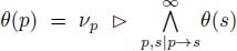. This relation expresses the fact that an ∞ – steep path of p passes through a neighboring node s verifying p → s, for which θ(s) is minimum. In the next chapter, we create an ∞ – steep digraph associated with any node-weighted graph by flooding, starting from its black holes and creating arcs along the propagation of the flood.