13
Two Paradigms for Creating a Partition or a Partial Partition on a Graph

13.1. Summary of the chapter

This chapter discusses the relative merits of partitions versus dead leaves models. In a watershed partition, each node is assigned to the catchment basin of one and only one black hole. Catchment basins do not overlap and form a partition of the domain. The problem is that obtaining such a partition is not possible without some arbitrary choices between alternative assignments to distinct black holes. In fact, even in an ∞ – steep digraph, catchment zones may still overlap, and we have to decide, for each node in an overlapping zone, to which catchment basin it has to be attributed. Many more or less arbitrary ways to do these assignments exist.

Another model is a dead leaves model, which also produces a partition but is able to recognize the zones where catchment zones overlap. In a dead leaves model, the labels are assigned priorities and the catchment zones are stacked on top of one another, the most prioritary ones covering the less prioritary ones. In conjunction with the arcs of the digraph, it is then possible to recognize nodes belonging to overlapping zones, since such nodes hold a label but are the origin of an arc towards a node with a different label, with a lower priority. This property will be used to construct segmentation strategies in which the first stage produces a dead leaves model with overlapping zones. The second stage then reduces or suppresses the overlapping zones we choose to resegment.

13.2. Setting up a common stage for node- and edge-weighted graphs

We have shown the deep relationships between node- and edge-weighted graphs. The trajectories of a drop of water gliding from node to node along flowing paths are identical. Moreover, it is possible to associate a node-weighted flow digraph with each node- or edge-weighted graph, in which each arrow represents a possible motion of a drop of water from the origin to the extremity of the arrow. The flowing paths of the initial graph simply become directed paths in the derived digraphs.

For a node-weighted graph, G(ν, nil) an arrow (p → q) is created from p to q in the digraph if ν_p ≥ ν_q.

For an edge-weighted graph G(nil, η), all edges never crossed by a drop of water are first suppressed: they are all edges which are not the lowest edge of one of their extremities. The resulting pruned graph is ↓ G(nil, η). An arrow (p → q) is created from p to q in the digraph ↓, if e_pq is one of the lowest edges of p. Such an edge verifies ν_p ≥ ν_q for the weight distribution ν = ε_neη.

As a result, whatever the initial graph, we have to study the topography of a node-weighted digraph , in which (p → q) iff ν_p ≥ ν_q.

Several tools have been defined to simplify such digraphs and various topographical structures derived from them.

13.3. A brief tool inventory

13.3.1. Operators making no use of the node weights

On the digraph , we define:

1. – the downstream and the upstream of a node or a group of nodes;
2. – flat zones, made of isolated nodes without outgoing arrow, or connected subgraphs in which couples of neighboring nodes are linked by a double arrow ⇆;
3. – black holes are flat zones without outgoing arcs;
4. – catchment zones are the upstream of the black holes.

13.3.2. Operators propagating labels

Labels assigned to some nodes or group of nodes may be propagated upstream or downstream. A priority relation is defined between the labels. If a node is suitable to receive several labels, it is assigned the most prioritary label.

13.3.3. Operators making use of the node weights and the graph structure

13.3.3.1. The core-expanding algorithm

The core-expanding algorithm constructs a partition of the nodes in catchment basins, i.e. catchment zones with minimum overlapping. It uses the node weights and the arrows of the digraph. It propagates the labels of the minima along the ∞ — steep flowing paths; the steepness of a flowing path being the list of its node weights. A lexicographic order relation between these lists is used to compare the steepness of the paths.

There also exists a version of this algorithm working on a graph and not on a digraph. It works on G(ν, nil) if the initial graph is a node-weighted graph or on ↓G(ε_neη, nil) if the initial graph is an edge-weighted graph.

13.3.3.2. The pruning algorithm

A pruning operator has also been defined, which is able to prune the digraph and cut the first edge of each path whose steepness is below some threshold. If the pruning operator is applied up to convergence, only ∞ — steep paths remain.

13.4. Dead leaves tessellations versus tilings: two paradigms

Watersheds have appeared as a powerful segmentation tool in image processing. It is able to create a partition of the nodes of a graph into regions, each containing a regional minimum. In the classical definition of a watershed, each catchment basin is the zone of influence of a regional minimum for a particular distance function, as, for instance, the topographical distance function. The core-expanding algorithm presented earlier is a shortest distance algorithm able to construct the Voronoï tessellation associated with the topographic distance. If we use a hierarchical queue for scheduling the algorithm, the distance is, in fact, a lexicographic distance, and the labels of the minima are propagated along ∞ — steep flowing paths. Ideally, each node should be assigned to the regional minimum, which is closest for the distance considered. In fact, for each distance which is used, a few nodes exist that are at the same distance of 2 minima, and some tie-braking mechanism has to be used.

The approach based on pruning the graph does not intentionally create such a fair sharing of the nodes between the regional minima. It also constructs a partition, in which each region contains a regional minimum. However, this partition is a dead leaves tessellation of catchment zones, covering each other, according to some priority rule between labels. If a node belongs to two or more catchment zones, it receives the label with the highest priority. The regional minima appear nevertheless in the dead leaves tessellation as a regional minimum never belongs to the catchment zone of another minimum.

The resulting dead leaves tessellation is all but fair, as the nodes belonging to two catchment zones are all assigned to the catchment zone with the highest priority label. The situation worsens if we construct the catchment zones of the regional minima on the initial digraph without pruning it. With increasing degrees of pruning, the catchment zones indeed become smaller, overlapping less with each other. For an ∞ — pruning, that is, a pruning up to the stability of the digraph is the overlapping minimal, equivalent to the overlapping produced by the core-expanding algorithm scheduled by a hierarchical queue.

In this section, we examine when and why one approach should be favored above the others, or how both may be combined advantageously.

13.5. Extracting catchment zones containing a particular node

13.5.1. Core expansion versus pruning algorithms

Suppose that we aim to extract the catchment zone containing a particular node p in a flow digraph.

The first solution is based on the core-expanding algorithm. The regional minima of the digraph are detected and labeled. The core-expanding algorithm creates a partition of the nodes, in which each catchment basin contains one regional minimum and holds the label of the minimum. The catchment zone containing the node p is then easily extracted. The node p is then assigned to one and only one catchment zone.

The second solution based on pruning first prunes the digraph, more or less severely. The pruning operator ↓^k cuts the first arc of each flowing path, which is not at least k — steep.

The node p is assigned a label which is propagated downstream in the pruned digraph. The node p may belong to one or several catchment zones of the pruned graph. The flowing paths that have their origin in p end in the regional minima of this catchment zone, if it is unique, or these catchment zones if they are several of them. In the final step, the label of the labeled regional minimum or minima is propagated upstream, labeling the catchment zone or zones containing the node p.

When the intensity k of the pruning increases, the catchment zones get smaller. It is then possible that, for a small value of k, the node p belongs to several catchment zones and only to one for a higher degree of pruning.

13.5.2. Illustration of the pruning algorithm

13.5.2.1. Illustration on a small grid

We illustrate the pruning effect on the downstream of a node and the catchment zones containing it with two examples.

In Figure 13.1 we have three images in each row: on the left a gray tone image and in the center a digraph, in which a node p has been marked in red, its downstream in blue and the ending regional minimum in green. On the right, we have added in gray the upstream of the downstream, i.e. the catchment zone containing p. The first row presents the initial gray tone image ν in Figure 13.1(a) and the associated 2-steep flow digraph 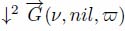in Figure 13.1(b), in which arcs link each node with its lowest neighbors.

The next rows of Figure 13.1 present successive pruning of this digraph, the left image presenting the node weights and the central image the remaining arcs after pruning. The second, third and fourth rows, respectively, represent prunings ↓³, ↓⁴, ↓⁶: both the downstream zones of p as its catchment zone get smaller when the pruning gets more severe. In Figure 13.1(b,e), the downstream of p is the union of several flowing paths with p as the origin. In Figure 13.1(h,k), after prunings ↓⁴ and ↓⁶, the downstream of p is reduced to a single flowing path, the same for both prunings. The catchment zones of p are also identical for prunings ↓⁴ and ↓⁶ and are smaller than the catchment zones obtained for the prunings ↓² and ↓³. This example shows that the pruning ↓⁴ is in this case already sufficient for obtaining optimal results. In other situations, more intense pruning may be required.

13.5.2.2. Illustration of a digital elevation model

The same operation is now made on an image representing a real topographic surface, namely a digital elevation model of a mountainous region with many rivers. Figure 13.2(a) presents a digital elevation model, with which (after some preprocessing as explained below) an ∞ — steep digraph has been associated. In Figure 13.2(b), the labels of these nodes have been propagated upstream, highlighting the attraction zone of the nodes, i.e. all points from where a drop of water may reach the labeled nodes, following an ∞ — steep flowing line. In Figure 13.2(c), the labels of these nodes has been propagated downstream, highlighting the rivers reached by the flowing path starting from the labeled nodes. These rivers end at a regional minimum of the image and assign their label to the regional minimum. Finally, Figure 13.2(d) presents the upstream of the labeled regional minima, i.e. the catchment zones that contain the marked nodes.

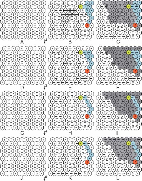
Figure 13.1. The downstream and upstream of the red node in the same digraph after increasing pruning intensities to equal 2,3,4 and 6. The left image presents the node weigths, the central image the downstream propagation of the red node and the right image the catchment zone of the red node, obtained by upstream propagation of the downstream. For a color version of the figures in this chapter, see www.iste.co.uk/meyer/topographical1.zip

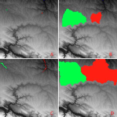
Figure 13.2. a) A digital elevation model in which a green and a red dot have been hand marked. b) The upstream of the marked nodes, with the same color. c) The downstream of the marked nodes follows a river leading outside of the domain, towards the sea. d) The downstream of the upstream represents the catchment zone of both marked nodes. The catchment zone holding the label with the highest priority covers the catchment zone with a lower priority. Here, the red label has a higher priority than the green label

13.6. Catchment zones versus catchment basins

In Chapter 14, we show how to combine and take advantage of both methods.

The core-expanding algorithm is extremely efficient but rigid: the labels of all regional minima have to be propagated in parallel, the extension of a catchment basin being stopped by the extension of a neighboring catchment basin.

On the contrary, pruning the digraph is the source of great flexibility: upstream or downstream propagation of labels may be done locally, in any order. Each catchment zone may take its full extension, independently of all other catchment zones, if it does not overlap with others. In the case of overlapping, the catchment zones will be covered with higher prioritary labels and cover those with a lower priority.

The same happens in the case of the downstream propagation of labels, which is subject to the same priority rule between labels.

Every time a node is suitable to take several labels, it takes the most prioritary one, independently of the order with which these labels are proposed.

These good properties are true for any flow digraph, independently of the degree of pruning that has been applied to it. However, acceptable results are only obtained after suitable pruning.

The next chapters illustrate the power and flexibility offered by the use of catchment zones.