15
Propagating Segmentations

15.1. Summary of the chapter

In section 15.2, we show how an image with sufficient contrasted objects may be segmented region-by-region. Every time a catchment zone has been fully reconstructed, we extract the neighboring catchment zone, separated from the previous one by the lowest pass point.

In section 15.3, we show how it is possible to adapt this method to marker-based segmentation.

15.2. Step-by-step segmentation

15.2.1. Principle of the method

We consider a node-weighted graph and its associated flowing digraph, after its pruning by ↓^k. We suppose that the graph has already been partially segmented: a part of the domain has been segmented and another part not yet. We suppose that the segmented region is a union of catchment zones of the flowing graph.

We aim to extend the segmented domain in a stepwise fashion. We search for the lowest pass point on the boundary of the already segmented region, using the method presented in the chapter “intermezzo”. We consider all edges that have one extremity in the segmented region and the other extremity outside. We assign to each of these edges the maximal weight of its extremities. We then search for the edge (or one of the edges if there are more than one) with the smallest weight. If e_pq is this edge, p belonging to the segmented region and q being outside, we assign to the node q a label, which may be chosen as follows:

1. – rule 1: we assign to q a new label, q being the germ of a new region;
2. – rule 2: we assign to q the label of p, allowing a stepwise marker-based segmentation. The catchment zone of q is absorbed by the catchment zone of p.

We then extract the catchment zone containing q, extending the segmented zone. We call this procedure “lowest neighbor segmentation”.

We now present several examples where this step-by-step segmentation method is applied.

15.2.2. Segmentation of blood cells

Figure 15.1(a) presents an image f with blood cells, namely a lymphocyte surrounded by erythrocytes. The image is well contrasted and the background is clean. We start with one marked node in the background and progressively segment the whole scene.

The gradient image ∂f is constructed and filtered (see Figure 15.1(b)) (the image ∂f is submitted to the highest flooding below a ceiling function obtained by adding a constant value to ∂f). Thus, the chromatin structures within the lymphocytes almost disappear from the gradient image.

The flow digraph associated with the gradient image is constructed and submitted to a pruning ↓⁵. We introduce a seed point in the background of the image (it appears in red in Figure 15.1(b), superimposed with the gradient image). The catchment zone containing the seed point is extracted and assigned a label, appearing in red color in Figure 15.1(e). It contains the part of the background which is accessible. We then iteratively apply the “lowest neighbor segmentation” procedure until all nodes are labeled. We give a new label to each new segmented region.

Figures 15.1(f,g,h) show the progression of the segmentation, each iteration adding one region. We recognize that the process has converged when no nodes remain without label.

We consider again the filtered gradient image represented in Figure 15.1(b). Its labeled regional minima are visible in Figure 15.1(c). The associated watershed partition constructed with the core expanding algorithm is presented in Figure 15.1(d) and appears quite similar with the partition created by the step-by-step segmentation in Figure 15.1(h).

The results obtained by both methods are similar.

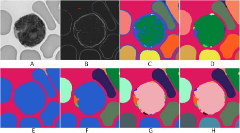
Figure 15.1. a) Initial image of a lymphocyte and of erythrocytes. b) Filtered gradient image and marker (in red) in the background. c) Regional minima of the filtered gradient image. d) Watershed partition obtained by the core-expanding algorithm. e) The flooding digraph associated with the gradient image is constructed and submitted to a pruning ↓⁵. The marked catchment zone is extracted, corresponding to the largest part of the background between the cells. f) The lowest transitions zone along the contour has been found and the corresponding catchment zones extracted. g) Result after two more steps of the same algorithm. h) The final result is obtained after five iterations of the algorithm, following the extraction of the first catchment zone to be compared with image D, obtained by the core-expanding algorithm. For a color version of the figures in this chapter, see www.iste.co.uk/meyer/topographical1.zip

In conclusion, this method creates a dead leaves tessellation of the image without significant errors if the initial pruning is intense enough and if the transitions between the objects of the scene are well marked.

15.2.3. Segmentation of an electronic circuit

We present here another example of an image with well-marked transitions between structures and substructures in the image, and without noise. The step-by-step segmentation method presented above also works well on this example. Figure 15.2 presents an image of an electronic circuit where the background is black and the wires are bright. The wires themselves present substructures, at the overlapping zones of two wires, which are more bright. The first two images in the series present the initial image f and its gradient ∂f. In both of them, we have indicated a seed point in red. The flow digraph associated with the gradient image is constructed and submitted to a pruning ↓³. The catchment zone containing the seed point is constructed and assigned a label, appearing in red color. We then iteratively apply the “lowest neighbor segmentation” until the complete wire is extracted; this produces the images 15.2(c,d,e,f) and (g). Without stopping criterion, the whole image would be reconstructed. The last image (see Figure 15.2(h)) shows what happens when the wire is reconstructed: a new region with a yellow label, belonging to the background jumps outside the wire, is extracted.

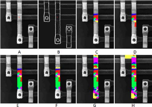
Figure 15.2. Progressive extraction of the catchement zones starting from a seed point

The intensity of the transition between a newly segmented catchment zone and the portion of the image segmented previously is measured by the altitude of the pass point between the two regions. In our case, the transition between this yellow region and the wire is significantly higher than the transitions inside the wire, indicating that the segmentation of the first wire is complete.

The transitions between neighboring catchment zones do not have the same intensity. Some zones are extremely similar in the initial image, and the gradient between them has a low value. Other transitions are higher, marking the transition between the substructures of a given wire or even higher when they mark the transition between the wire and the background. If we change the labels only when a significantly larger transition is observed, compared with the previous and the next transition, we are able to detect the substructure of the wire. The successive transitions for the first regions that have been reconstructed are as follows: 13, 14, 20, 13, 40 and 20. The value 40 is significantly higher than the transition before and the transition after. It corresponds to the red region detected in Figure 15.3(c). We will encode it by (i = 5: 13 40 20), where i represents the rank of a high transition, followed by the triple of points marking the transition). The five highest transitions similarly encoded are: (i = 5: 13 40 20)(i =11: 27 61 13)(i =14: 14 40 13)(i =16: 30 47 41)(i =20: 34 67 14). Changing the color of the label at each of these transitions yields the segmentation in six regions of the wire presented in Figure 15.3(c). Changing the label only at the highest transition (i =20: 34 67 14) yields the segmentation in Figure 15.3(d). The limits of the wire itself compared to the background are expressed by a much higher transition (i =29: 27 141 60) and correspond to the moment where the background starts to be invaded in Figure 15.2(h). This success of this method is due to high contrasts and low noise in the image.

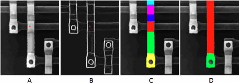
Figure 15.3. Extraction of the regions corresponding to the highest transitions in the gradient image between regions

15.3. Marker-based segmentation

The step-by-step extension of a segmented region may also serve for marker-based segmentation. The initial segmentation is obtained by defining several markers, i.e. labels given to some nodes, which will serve as seeds for the subsequent segmentation. Figure 15.4(a) and (b), respectively, presents an image to be segmented and its filtered gradient. In Figure 15.4(c), several markers have been drawn manually.

A flowing digraph associated with the gradient image is created and pruned by ↓⁵. The initial segmentation is obtained by downwards propagation of the labels of Figure 15.4(c), yielding Figure 15.4(d).

We then iteratively apply the “lowest neighbor segmentation” in which we propagate the labels from region to region (we apply rule 2, assigning to the new seed node q the label of its already segmented neighboring node p). Figure 15.4(e) shows the result after seven iterations and Figure 15.4(f) after convergence.

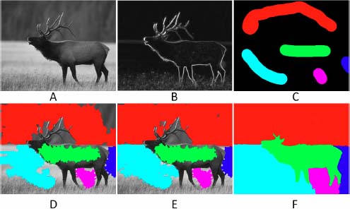
Figure 15.4. Marker-based segmentation by a stepwise propagation of the markers: a) Image to be segmented. b) Filtered gradient image. c) Hand-drawn markers. d) Initial segmentation by propagating the labels of the markers on the 5 – steep digraph associated with the gradient image. e) After repeating seven times the step-by-step segmentation. f) After convergence