Chapter 9

Coordinate Geometry

Chapter Check-In

Coordinate graphs

Graphing equations on coordinate planes

Slope and intercept of linear equations

Finding equations of lines

Linear inequalities and half-planes

Coordinate geometry deals with graphing (or plotting) and analyzing points, lines, and areas on the coordinate plane (coordinate graph).

Coordinate Graphs

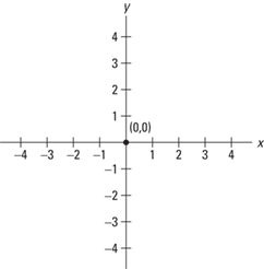
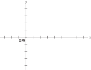
Each point on a number line is assigned a number. In the same way, each point in a plane is assigned a pair of numbers. These numbers represent the placement of the point relative to two intersecting lines. In coordinate graphs (see Figure 9–1), two perpendicular number lines are used and are called coordinate axes. One axis is horizontal and is called the x-axis. The other is vertical and is called the y-axis. The point of intersection of the two number lines is called the origin and is represented by the coordinates (0, 0).

Figure 9–1 An x-y coordinate graph.

Each point on a plane is located by a unique ordered pair of numbers called the coordinates. Some coordinates are noted in Figure 9–2.

Figure 9–2 Graphing or plotting coordinates.

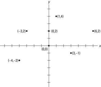
Notice that on the x-axis numbers to the right of 0 are positive and to the left of 0 are negative. On the y-axis, numbers above 0 are positive and below 0 are negative. Also, note that the first number in the ordered pair is called the x-coordinate, or abscissa, and the second number is the y-coordinate, or ordinate. The x-coordinate shows the right or left direction, and the y-coordinate shows the up or down direction.

The coordinate graph is divided into four quarters called quadrants. These quadrants are labeled in Figure 9–3.

Figure 9–3 Coordinate graph with quadrants labeled.

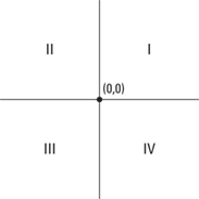
Notice the following:

In quadrant I, x is always positive and y is always positive.

In quadrant II, x is always negative and y is always positive.

In quadrant III, x and y are both always negative.

In quadrant IV, x is always positive and y is always negative.

Graphing equations on the coordinate plane

To graph an equation on the coordinate plane, find the coordinate by giving a value to one variable and solving the resulting equation for the other value. Repeat this process to find other coordinates. (When giving a value for one variable, you could start with 0, then try 1, and so on.) Then graph the solutions.

Example 1: Graph the equation x + y = 6.

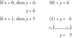
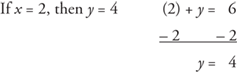
Using a simple chart is helpful.

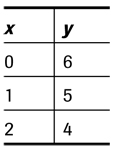
Now plot these coordinates as shown in Figure 9–4.

Figure 9–4 Plotting of coordinates (0,6), (1,5), (2,4)

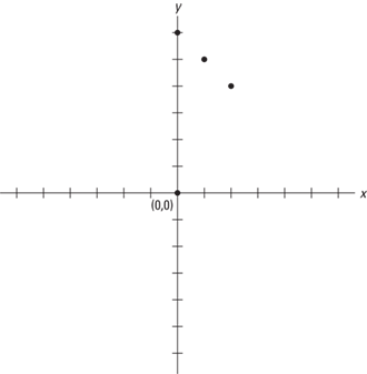
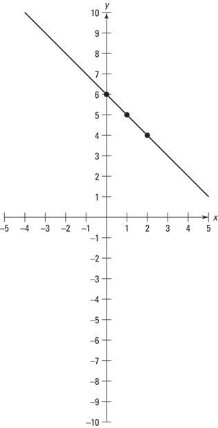
Notice that these solutions, when plotted, form a straight line. Equations whose solution sets form a straight line are called linear equations. Complete the graph of x + y = 6 by drawing the line that passes through these points (see Figure 9-5).

Figure 9–5 The line that passes through the points graphed in Figure 9–4.

Equations that have a variable raised to a power, show division by a variable, involve variables with square roots, or have variables multiplied together will not form a straight line when their solutions are graphed. These are called nonlinear equations.

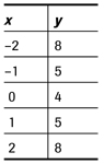
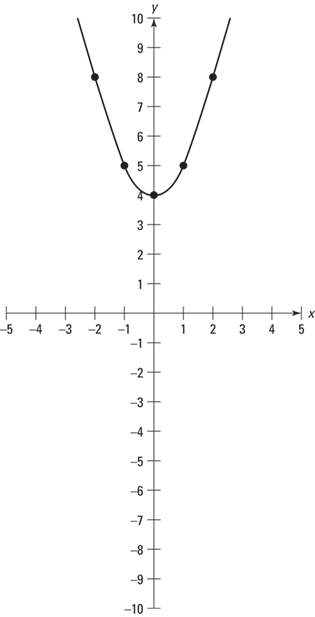
Example 2: Graph the equation y = x2 + 4.

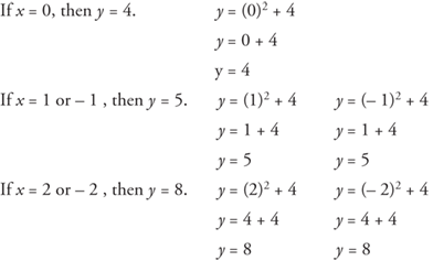
Use a simple chart.

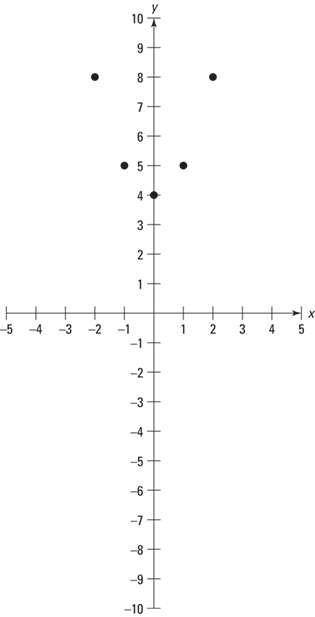
Now plot these coordinates as shown in Figure 9–6.

Notice that these solutions, when plotted, do not form a straight line.

These solutions, when plotted, give a curved line (nonlinear). The more points plotted, the easier it is to see and describe the solutions set.

Figure 9–6 Plotting the coordinates in the simple chart.

Complete the graph of y = x2 + 4 by connecting these points with a smooth curve that passes through these points (see Figure 9–7).

Figure 9–7 The line that passes through the points graphed in Figure 9–6.

Slope and intercept of linear equations

There are two relationships between the graph of a linear equation and the equation itself that must be pointed out. One involves the slope of the line, and the other involves the point where the line crosses the y-axis. In order to see either of these relationships, the terms of the equation must be in a certain order.

(+)(1)y = ( )x + ( )

When the terms are written in this order, the equation is said to be in y-form. Y-form is written y = mx + b, and the two relationships involve m and b.

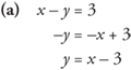
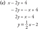
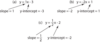
Example 3: Write the equations in y-form.

(b) y = –2x + 1 (already in y-form)

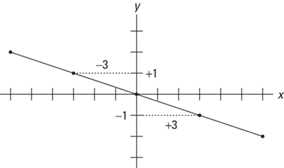
As shown in the graphs of the three problems in Figure 9–8, the lines cross the y-axis at –3, +1, and –2, the last term in each equation.

If a linear equation is written in the form of y = mx + b, b is the y-intercept.

The slope of a line is defined as

and the word “change” refers to the difference in the value of y (or x) between two points on the line.

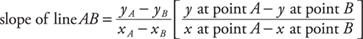
Note: Points A and B can be any two points on a line; there will be no difference in the slope.

Figure 9–8 Graphs showing the lines crossing the y-axis.

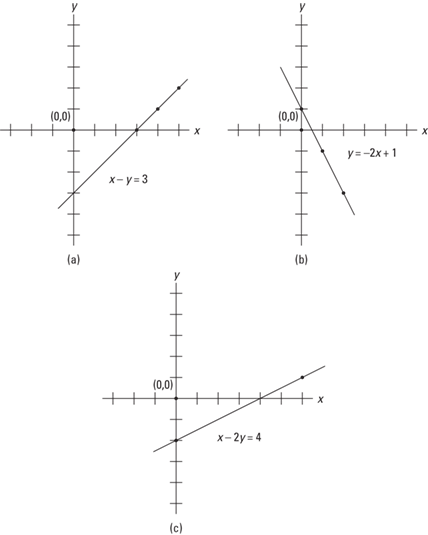
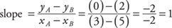
Example 4: Find the slope of x – y = 3 using coordinates.

To find the slope of the line, pick any two points on the line, such as A (3, 0) and B (5, 2), and calculate the slope.

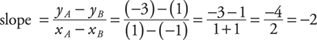
Example 5: Find the slope of y = –2x – 1 using coordinates.

Pick two points, such as A (1, –3) and B (–1, 1), and calculate the slope.

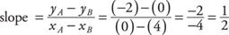
Example 6: Find the slope of x – 2y = 4 using coordinates.

Pick two points, such as A (0, –2) and B (4, 0), and calculate the slope.

Looking back at the equations for Example 3(a), (b), and (c) written in y-form, it should be evident that the slope of the line is the same as the numerical coefficient of the x-term.

Graphing linear equations using slope and intercept

Graphing an equation by using its slope and y-intercept is usually quite easy.

1. State the equation in y-form.

2. Locate the y-intercept on the graph (that is, one of the points on the line).

3. Write the slope as a ratio (fraction) and use it to locate other points on the line.

4. Draw the line through the points.

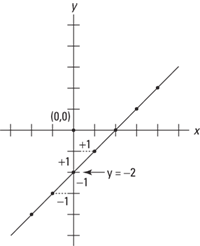
Example 7: Graph the equation x – y = 2 using slope and y-intercept.

Locate –2 on the y-axis and from this point count as shown in Figure 9–9:

slope = 1

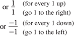
Figure 9–9 Graph of line y = x – 2.

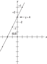
Example 8: Graph the equation 2x – y = –4 using slope and y-intercept.

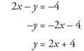
Locate +4 on the y-axis and from this point count as shown in Figure 9–10:

slope = 2

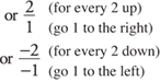
Figure 9–10 Graph of line 2x – y = –4.

Example 9: Graph the equation x + 3y = 0 using slope and y-intercept.

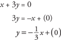
Locate 0 on the y-axis and from this point count as shown in Figure 9–11:

slope =

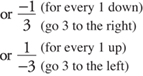
Figure 9–11 Graph of line x + 3y = 0.

Finding the equation of a line

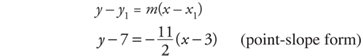
To find the equation of a line when working with ordered pairs, slopes, and intercepts, use one of the following approaches depending on which form of the equation you want to have. There are several forms, but the three most common are the slope-intercept form, the point-slope form, and the standard form. The slope-intercept form looks like y = mx + b where m is the slope of the line and b is the y-intercept. The point-slope form looks like y – y1 = m(x – x1) where m is the slope of the line and (x1,y1) is any point on the line. The standard form looks like Ax + By = C where, if possible, A, B, and C are integers.

Method 1. Slope–intercept form.

1. Find the slope, m.

2. Find the y-intercept, b.

3. Substitute the slope and y-intercept into the slope-intercept form, y = mx + b.

Method 2. Point-slope form.

1. Find the slope, m.

2. Use any point known to be on the line.

3. Substitute the slope and the ordered pair of the point into the point-slope form, y – y1 = m(x – x1).

Note: You could begin with the point-slope form for the equation of the line and then solve the equation for y. You will get the slope-intercept form without having to first find the y-intercept.

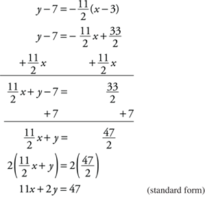
Method 3. Standard form.

1. Find the equation of the line using either the slope-intercept form or the point-slope form.

2. With appropriate algebra, arrange to get the x-terms and the y-terms on one side of the equation and the constant on the other side of the equation.

3. If necessary, multiply each side of the equation by the least common denominator of all the denominators to have all integer coefficients for the variables.

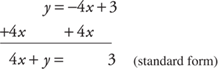
Example 10: Find the equation of the line, in slope-intercept form, when m = – 4 and b = 3. Then convert it into standard form.

1. Find the slope, m.

m = – 4 (given)

2. Find the y-intercept, b.

b = 3 (given)

3. Substitute the slope and y-intercept into the slope-intercept form, y = mx + b.

y = – 4x + 3 (slope-intercept form)

4. With appropriate algebra, arrange to get the x-terms and the y-terms on one side of the equation and the constant on the other side of the equation.

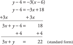
Example 11: Find the equation of the line, in point-slope form, passing through the point (6, 4) with a slope of –3. Then convert it to standard form.

1. Find the slope, m.

m = –3 (given)

2. Use any point known to be on the line.

(6, 4) (given)

3. Substitute the slope and the ordered pair of the point into the point-slope form,

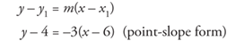
4. With appropriate algebra, arrange to get the x-terms and the y-terms on one side of the equation and the constant on the other side of the equation.

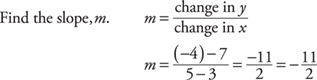
Example 12: Find the equation of the line, in either slope-intercept form or point-slope form, passing through (5, –4) and (3, 7). Then convert it to standard form.

Starting with slope-intercept:

1.

2. Find the y-intercept, b.

Substitute the slope and either point into the slope-intercept form.

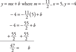
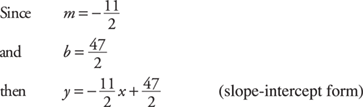
3. Substitute the slope and y-intercept into the slope-intercept form, y = mx + b.

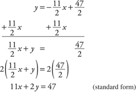
4. With appropriate algebra, arrange to get the x-terms and the y-terms on one side of the equation and the constant on the other side of the equation.

If necessary, multiply each side of the equation by the least ­common denominator of all the denominators to have all integer coefficients for the variables.

Starting with point-slope form:

1.

2. Use any point known to be on the line.

(3, 7) (given)

3. Substitute the slope and the ordered pair of the point into the point-slope form,

4. With appropriate algebra, arrange to get the x-terms and the y-terms on one side of the equation and the constant on the other side of the equation.

If necessary, multiply each side of the equation by the least ­common denominator to have all integer coefficients for the variables.

Linear Inequalities and Half-Planes

Each line plotted on a coordinate graph divides the graph (or plane) into two half-planes. This line is called the boundary line (or bounding line). The graph of a linear inequality is always a half-plane. Before graphing a linear inequality, you must first find or use the equation of the line to make a boundary line.

Open half-plane

If the inequality is a “>” or “<”, then the graph will be an open half-plane. An open half-plane does not include the boundary line, so the boundary line is written as a dashed line on the graph.

Example 13: Graph the inequality y < x – 3.

First graph the line y = x – 3 to find the boundary line (use a dashed line, since the inequality is “<”) as shown in Figure 9–12.

Figure 9–12 Graph of boundary line for y < x – 3.

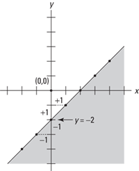
Now shade the lower half-plane as shown in Figure 9–13, since y < x – 3.

Figure 9–13 Graph of inequality y < x – 3.

To check to see whether you’ve shaded the correct half-plane, plug in a pair of coordinates—the pair of (0, 0) is often a good choice. If the coordinates you selected make the inequality a true statement when plugged in, then you should shade the half-plane containing those coordinates. If the coordinates you selected do not make the inequality a true statement, then shade the half-plane not containing those coordinates.

Since the point (0, 0) does not make this inequality a true statement,

y < x – 3

0 < 0 – 3 is not true.

You should shade the side that does not contain the point (0, 0).

This checking method is often simply used as the method to decide which half-plane to shade.

Closed half-plane

If the inequality is a “≤”or “≥”, then the graph will be a closed half-plane. A closed half-plane includes the boundary line and is graphed using a solid line and shading.

Example 14: Graph the inequality 2x – y ≤ 0.

First transform the inequality so that y is the left member.

Subtracting 2x from each side gives

–y ≤ –2x

Now dividing each side by –1 (and changing the direction of the inequality) gives

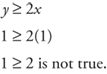
y ≥ 2x

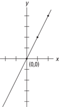
Graph y = 2x to find the boundary (use a solid line, because the inequality is “≥”) as shown in Figure 9–14.

Figure 9–14 Graph of the boundary line for y ≥ 2x.

Since y ≥ 2x, you should shade the upper half-plane. If in doubt, or to check, plug in a pair of coordinates. Try the pair (1, 1).

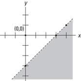
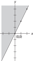
So you should shade the half-plane that does not contain (1, 1) as shown in Figure 9–15.

Figure 9–15 Graph of inequality y ≥ 2x.

Chapter Check-Out

1. Is x2 – 8 = y linear or nonlinear?

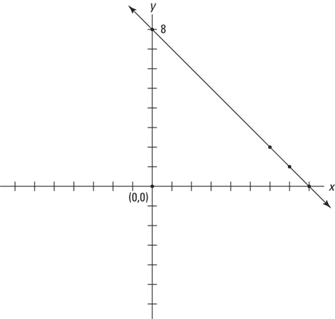
2. Graph: x + y = 8

3. Find the equation of the line, in point-slope form, passing through the point (6, 1) with a slope of –2. Then convert it to standard form.

4. Find the equation of the line, in slope-intercept form, passing through the points (–3, 4) and (2, –3). Then convert it to standard form.

5. Graph: y ≤ x – 2

Answers: 1. Nonlinear

2.

3. point-slope form: y – 1 = –2(x – 6); standard form: 2x + y = 13

4. slope-intercept form: ; standard form: 7x + 5y = –1

5.