Shapes

Plot the vertices of a regular 10-sided polygon, using the trigonometric functions sin() and cos() in the same way that you might generate a circle. Modify your code to generate a star by alternating long and short radii.1
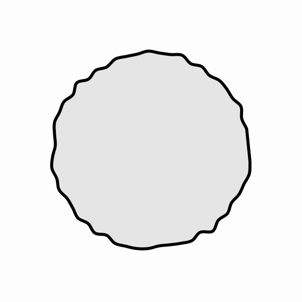
Plot the vertices of a many-sided polygon, using the functions sin() and cos() in the same way that you might generate a circle, but compute the position of each point with a radius that is slightly randomized. How closely can you make the result resemble a drop of ink?2
The numbers below define the vertices of a polygon. Write code that connects the dots to plot the shape. x={81, 83, 83, 83, 83, 82, 79, 77, 80, 83, 84, 85, 84, 90, 94, 94, 89, 85, 83, 75, 71, 63, 59, 60, 44, 37, 33, 21, 15, 12, 14, 19, 22, 27, 32, 35, 40, 41, 38, 37, 36, 36, 37, 43, 50, 59, 67, 71}; y={10, 17, 22, 27, 33, 41, 49, 53, 67, 76, 93, 103, 110, 112, 114, 118, 119, 118, 121, 121, 118, 119, 119, 122, 122, 118, 113, 108, 100, 92, 88, 90, 95, 99, 101, 80, 62, 56, 43, 32, 24, 19, 13, 16, 23, 22, 24, 20};
Axis-Aligned Minimum Bounding Box
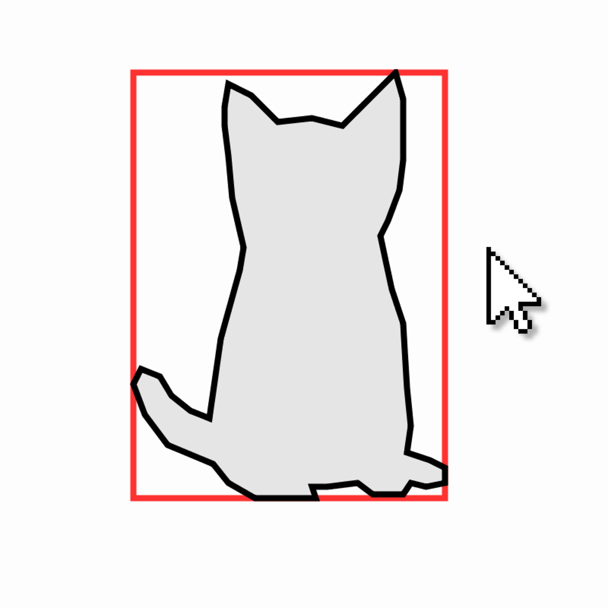
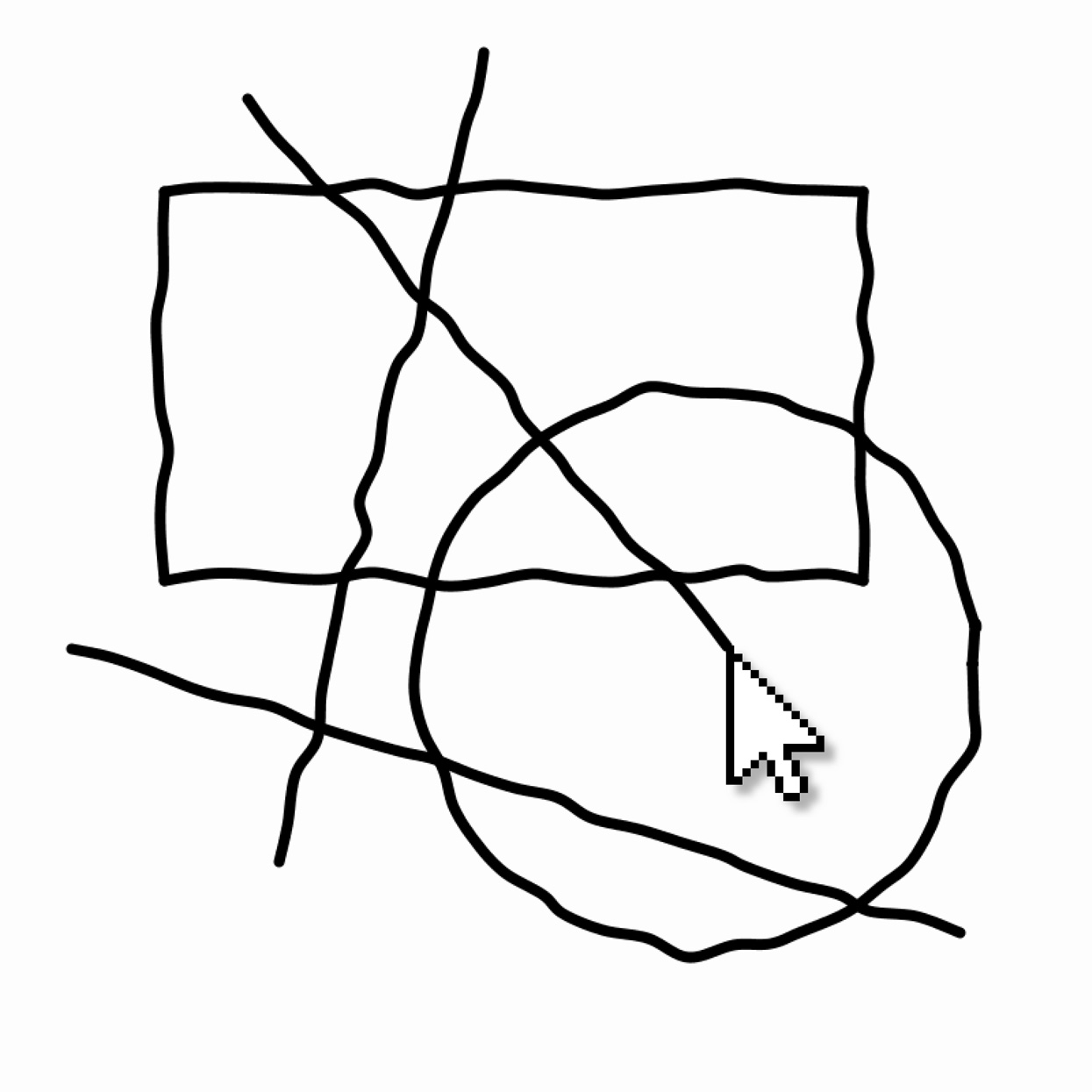
Given a 2D shape represented by a set of points, compute and plot its “bounding box”: a useful rectangle defined by the leftmost, rightmost, highest, and lowest points on the shape's contour. Create an interaction in which the shape is displayed differently if the cursor enters its bounding box.
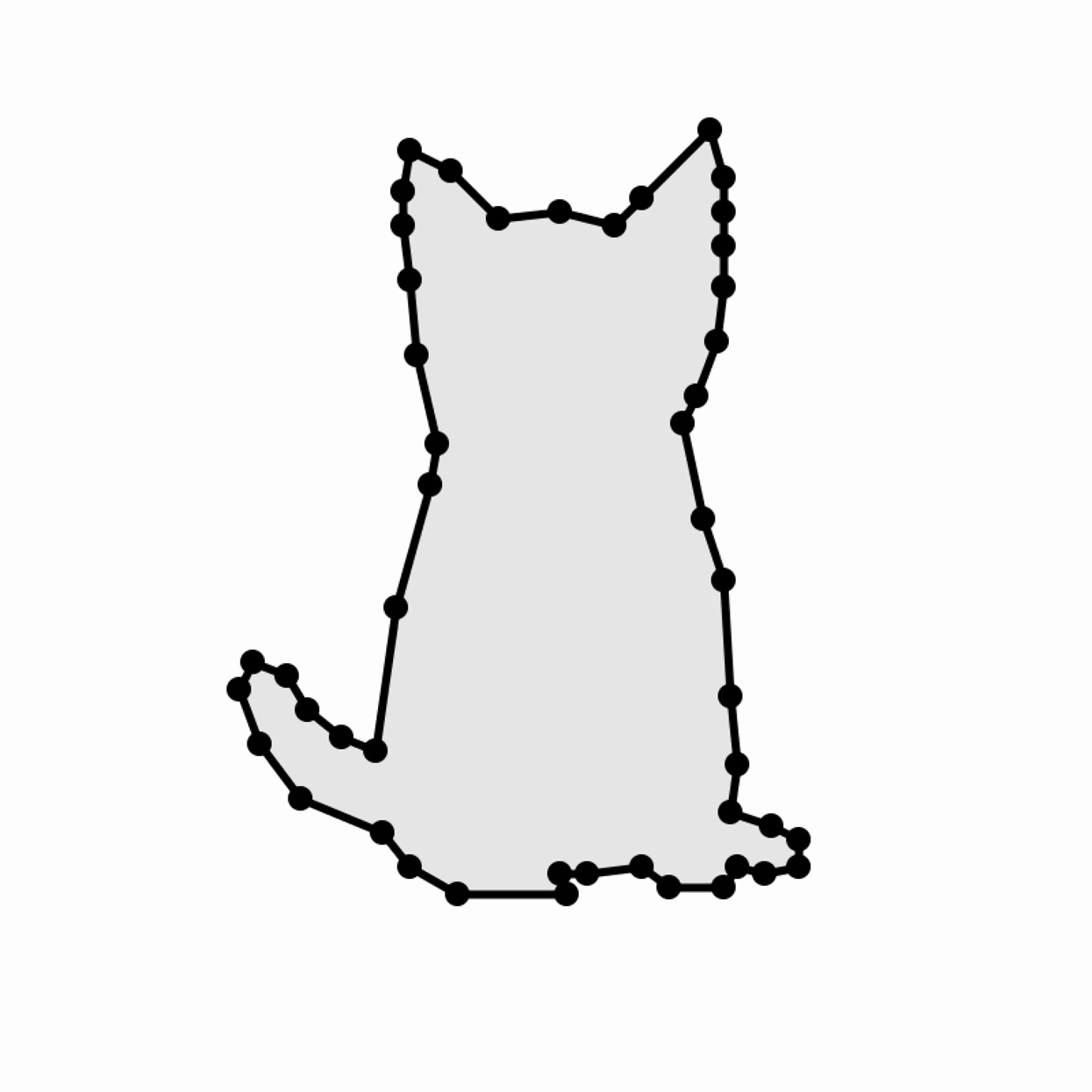
Given a 2D shape represented by a set of points, compute and plot the “centroid” of its outline—the location whose x-coordinate is the average of the x-coordinates of the points, and whose y-coordinate is the average of the y-coordinates of the points.
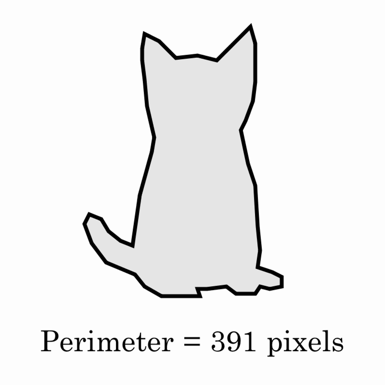
Given a 2D shape represented as a set of points, calculate the length (or perimeter) of its outline. To do this, add up the distances between every pair of consecutive points along its boundary. Don't forget to include the distance from the last point back to the first one.
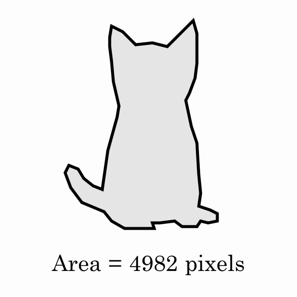
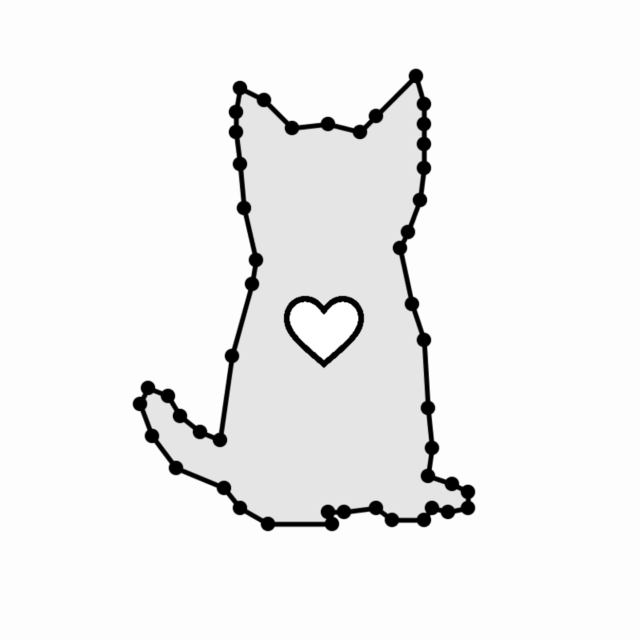
Given a simple (non-self-intersecting) 2D shape whose points are stored in arrays x[] and y[], calculate its area. This can be done using Gauss's area formula, or “shoelace algorithm,” which sums, for all points i, the products ((x[i+1] + x[i]) * (y[i+1] - y[i]))/2.0.
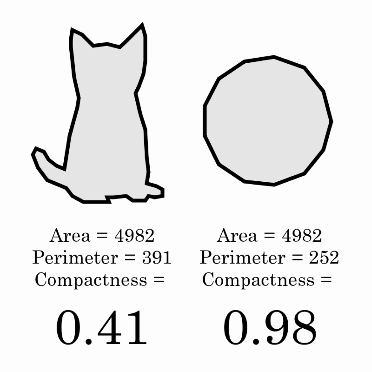
One of the simplest shape metrics is “compactness” (or isoperimetric quotient), which describes the extent to which a shape does or doesn't sprawl. Often used in redistricting to avoid gerrymandering, compactness is a dimensionless, scale-invariant, and rotation-invariant quantity.3 It is computed by taking the ratio of a shape's area to its squared perimeter. Compute the compactness of the provided shape. Compare this value with the compactness of some other shapes.
Detecting Points of High Curvature
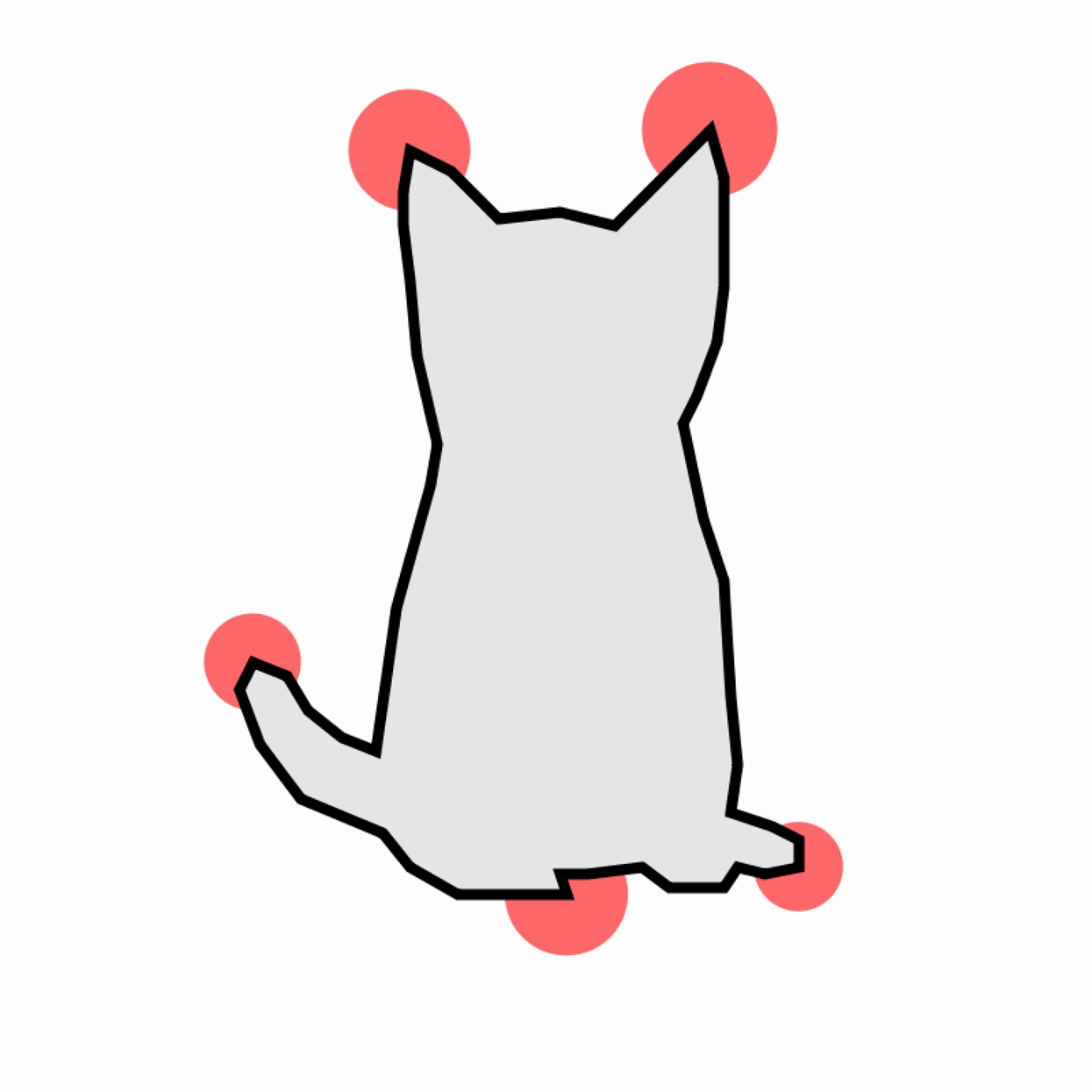
Given a 2D shape represented as a set of points, we can estimate the “local curvature” along the shape's boundary by computing the angle between consecutive trios of points. Using the provided shape, write code to determine which points have especially high curvature (i.e. the fingertips) and mark them with a colored dot. Hint: Use the dot product to compute the angles, and the cross product to distinguish positive curvature (convexities) from negative curvature (concavities).
Create a set of functions for rendering basic shapes with a hand-drawn feel. At a minimum, your library should provide functions for drawing line segments, ellipses, and rectangles.
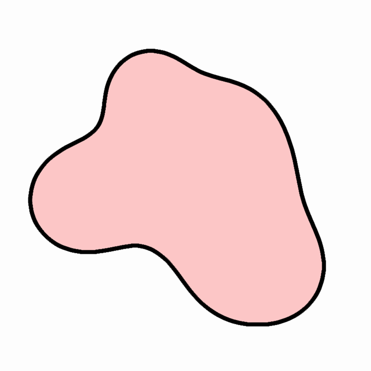
Using any means you prefer, design and animate an expressive 2D blob. For example: you could create a closed loop of Bézier curves; trace the contours of metaballs (implicit curves) using Marching Squares; calculate a Cassini ellipse, cranioid, or other parametric curve; or simulate a smooth ropelike contour using Verlet integration.