Replacing Darwin

Chapter 3

Cracking the Code

In a jigsaw puzzle, edge pieces constrain the arrangement of the center pieces. Since species are defined by their traits, the origin of traits constrains the puzzle of the origin of species. The origin of leopards and cheetahs depends on an answer to the origin of spots. The origin of toucans relies on the answer to the origin of large, colorful beaks. The origin of the blue whale is bound up in the origin of baleen. The origin of scorpions and the origin of stingers go hand in hand. The answer to the origin of traits represents the edge pieces to the puzzle.

In the previous chapter, we took steps toward understanding the origin of traits — but we did not reach the answer. For example, we observed the behavior of traits at the visible level and traced the control of this behavior to the DNA double helix. Nevertheless, we never uncovered how DNA controlled the behavior of traits.

The mystery of the how concealed the answers to several critical questions. Could the mechanism by which DNA controlled the behavior of traits be altered? Could it be changed to an entirely different program? Could leopards become whales? Could toucans change into scorpions? Could jellyfish become jaguars? The answers to these questions awaited the discovery of the mechanism by which DNA interfaced with traits.

Standing in the way of the answer were several paradoxes. First, in each generation, all traits are erased — only to be rebuilt again. This fact is a curious phenomenon in its own right. It’s one thing to observe red hair appear and disappear on a family tree. It’s something entirely different to discover that all traits — hair color, facial features, hands, legs, feet, etc. — are absent when sperm and egg meet, yet eventually appear in the adult.

Second, when this massive amount of change was compared to the theoretical changes involved in the origin of species, the paradox deepened. For example, consider some of the questions we have asked of species. Can a fish spawn a spider? Can elephants give birth to giraffes? Could butterflies sire birds? The differences between these pairs of creatures are striking — fins versus eight legs, trunks versus long necks, scaled wings versus feathered wings. The morphological changes required to transform one of these creatures into another are numerous. But none of these theoretical transformations are as profound as the transformations that occur during the process of development. For example, all of the species transformations listed above are between species with heads, trunks, limbs, respiratory systems, digestive systems, and excretory systems. To go from a single cell to, say, an adult zebra, far more visible change is required. At fertilization, head, trunk, limbs, etc. are absent.

Third, despite this enormous upheaval in morphology, the outcome of the developmental process was extremely consistent. Development of sperm and egg faithfully results in the same traits from generation to generation. In fact, it results in consistent species-specific traits. It must — or we would have no concept of species in our vocabulary. If each species could spawn something entirely different every generation, species wouldn’t be a scientific term.

Now consider again what it would take to form a new species. For a fish to become a spider, significant morphological changes must occur — an endoskeleton must transform into an exoskeleton, fins must become legs, an aquatic form of respiration must transform into a terrestrial form of respiration, etc. In other words, for new species to form, the developmental process would have to become less consistent.

Today, a small measure of developmental inconsistency occurs. Though the process of development produces a very consistent, species-specific outcome each generation, it doesn’t produce identical individuals each generation. For example, you differ from your parents. All three of you are clearly human, but you are not identical to your parents. As another example, no two zebra individuals are alike. Again, zebra parents and zebra offspring are both members of the same species, but none of the three are identical. A little bit of change happens each generation. But is the accumulation of these little changes over time enough to produce a new species?

The solution to these paradoxes held the key to discovering the origin of traits — the edge pieces to the puzzle — and the origin of species.

* * * *

Prior to the discovery of the DNA double helix, candidate solutions to these paradoxes began to emerge. One candidate arose from the fields of physics and chemistry. For example, consider the physics of transforming a single cell into a complex adult. This single cell would have to overcome many chemical and physical barriers in order to produce an adult. In other words, left to themselves, physical structures don’t spontaneously assemble into creatures with heads and tails. Instead, thanks to the Second Law of Thermodynamics,1 they degrade — much like an old library collects dust and eventually collapses without maintenance. To make a trunk or a long neck or a wing, cells would have to find a way to put energy into the system to overcome this thermodynamic barrier.

In the decades prior to the 1950s, the fundamental principles of cellular energy management began to be uncovered.2 The major players were proteins. Unlike human assembly and construction processes, cells don’t use electrical outlets or fossil fuels to power their division and growth. Instead, they utilize the sources available to them — nutrients in food stuffs. Once your stomach and intestines break down the meals you supply them (using, among other things, proteins to break down the food), the resultant chemical products are absorbed into the bloodstream (via protein channels, among other mechanisms) and passed on to cells where they are absorbed or transported inside (via proteins). In the womb, the developing and assembling baby receives these nutrients ultimately via the placental bloodstream.

Once inside the cell, more proteins break these tiny nutrients down into even smaller molecules. At the molecular level, sugars, fats, and other nutrients store an enormous amount of energy. The chemical bonds that hold the individual atoms of sugars and fats together can be broken. Doing so is an energetically favorable process — a process that proteins catalyze.

By analogy, food breakdown is like trying to roll a ball down a hill. Once you get the process started, natural forces like gravity takes over, and the ball picks up speed. Foodstuffs are like a ball sitting at the top of a hill.

However, to make the analogy more accurate, we’d need to put a little mound of dirt in front of the ball. With a little shove over the dirt, the ball will continue naturally on its own down the hill. But it won’t go down without a little shove. In the cell, chemical bonds in nutrients don’t immediately break. Because chemical “mounds of dirt” — in technical terms, activation energies — exist, chemical bonds aren’t spontaneously severed. Proteins3 help these processes get over the chemical “mounds of dirt.” Once started down this chemically favorable path, the chemical breakdown reactions continue (Figure 3.1).

The reverse process — resynthesizing these bonds — is energetically prohibitive. For the cell to assemble itself into an adult body with a trunk or long neck or wings, it has to make more fats, sugars, and whatever other molecules it needs to make these structures. Self-assembly is a very energetically challenging process. Again, by analogy, it’s like trying to roll the ball back up the hill. Going against gravity doesn’t happen naturally. It requires energetic input — your muscles, sweat, and hard work (Figure 3.1).

Alternatively, you might be able to get a ball up a hill by rolling it down another. If you give the ball a big enough push at the top of one hill, it might have enough energy to roll down one and then roll up another. Similarly, to become a full-grown adult, our single cell has to find a way to couple the energetically-favorable breakdown of food stuffs to the energetically-unfavorable synthesis of body parts (Figure 3.1).

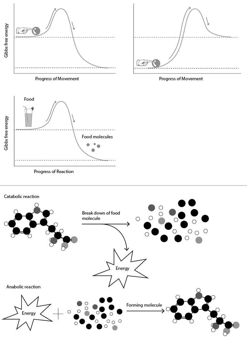
Figure 3.1. Illustration of basic cellular biochemical principles. Favorable chemical reactions in the cell can be compared to the process of rolling a ball down a hill. More realistically, they can be compared to rolling a ball over a small hump and then down a hill. These small humps represent activation energies, and proteins aid in reducing the size of this energetic barrier, allowing chemical reactions to proceed. Unfavorable chemical reactions can be compared to rolling a ball up a hill. Coupling these two rolling processes can allow unfavorable chemical reactions to proceed. In the cell, favorable chemical reactions (i.e., catabolic reactions) are coupled to unfavorable chemical reactions (i.e., anabolic reactions) via energy intermediates.

Proteins couple food breakdown to molecular synthesis. Not surprisingly, the process is complex. Several different types of nutrients get passed to cells (e.g., carbohydrates, proteins, fats). A mind-boggling number of individual chemical steps break down these various molecules to individual chemical components.

Theoretically, a single protein coupling machine could perform this task. In practice, it would have to be enormous in size — perhaps too enormous with respect to the size of a cell. Similarly, in building construction, humans don’t solve the energy coupling problem with a one-size-fits-all machine. We don’t have a single, massive structure at construction sites that pumps oil from the ground and then burns it in an engine that synthesizes concrete pillars, steel beams, windows, and dry wall. Instead, we refine the oil to gasoline at an oil refinery. A manufacturing plant assembles vehicles. The gasoline acts as an energy intermediate/currency that a wide variety of individual machines can use. A similar principle holds true for coal or nuclear power plants, except that the energy currency is electricity.

In the cell, division of labor also occurs. For example, many different proteins are involved in food breakdown. The result of this process is a form of energy currency. In the cell, the currency doesn’t take the form of gasoline or electrical outlets. Instead, it’s primarily in the form of a molecule called ATP (Figure 3.2; yes, it’s one of the nucleotides we encountered in the previous chapter). Then other proteins couple the breakdown of ATP to the synthesis of cell assembly products.

Figure 3.2. Adenosine triphosphate (ATP). Elements are represented with single letter abbreviations: carbon (C), nitrogen (N), oxygen (O), hydrogen (H), phosphorus (P). Ring structures (five sided, or joined five-sided and six-sided) consist entirely of carbon and hydrogen, unless otherwise indicated. Chemical bonds indicated by lines (single bond by one line; double bond by two lines). Subscripts denote number of atoms of the adjacent element. This structure is an RNA molecule (rather than a DNA molecule), as indicated by the extra “OH” linkage below the five-sided ring (highlighted with dashed arrow).

When we compare specific elements of this biological process to specific elements in the process of constructing a building, the cellular importance of proteins grows even larger. Both processes involve a nondescript starting point that transforms into a highly complex final result. Extending the analogy further, both construction projects need a way to transform energy and raw materials to something useful. Both need tools to connect the transformed energy and refined materials toward a desired end. At the building construction site, transformed energy and refined materials are taken for granted. We outsource these functions to power plants and manufacturing sites, respectively. Then we transport the products to the site. Tools are synthesized elsewhere and brought in as well. In contrast, the proteins of the cell act as the power plant, the factory, and the tools. Since the cell compartmentalizes these functions within itself, proteins do the jobs that humans spread out over a wide range.

Given the integral role that proteins had in transforming a non-descript single cell into an adult with diverse visible traits, proteins were a strong candidate for connecting DNA to the traits that define species.4

* * * *

For a single cell to self-assemble into an adult, what we’ve discussed is a good start to this process. But only a start. Transformed energy, manufactured materials, and powered tools (i.e., powered by ATP) are critical to getting the cell from zygote to birth. Yet, while these components are necessary, they aren’t sufficient.

If these things were all you had at a building construction site, you wouldn’t see your final product form. Dump transformed energy, manufactured materials, and powered tools in a pile, and a building won’t spontaneously assemble. Even if you send numerous construction crews, you can’t guarantee the outcome you desire — unless you have a blueprint that the crews agree to follow. Similarly, the cell needs a blueprint by which to control the activity of its powered protein tools.

In one sense, we already know where the blueprint lies. Since the visible appearance of a species is consistent from generation to generation, so also must the blueprint be. If this is true, then the blueprint must be heritable. Since the physical basis of heredity is DNA, we have an obvious candidate for the cellular blueprint.

But how could a linear series of nitrogenous bases in a twisted ladder-like structure specify a three-dimensional animal with a trunk, long necks, wings, or red hair? How could DNA organize the protein activity of the cell?

Figure 3.3. Sickle cell anemia. Among many normal blood cells, an abnormally shaped (sickle shaped) red blood cell is visible near the center of the image; the thin diagonal line points toward it.

The first answers took years of searching to find. The way in which DNA functions as the blueprint wasn’t discovered until over a decade after the structure of DNA was solved. Remarkably, despite requiring years of experimental investigation, the code was cracked before the DNA sequences of any creature were elucidated.5

However, the first hints to the relationship between DNA and protein long predated the discoveries of Watson and Crick. In 1902, the British physician Archibald Garrod documented several cases of a human metabolic disorder — one that turns the urine dark. The distribution of the cases hinted at Mendel’s principles, suggesting a genetic origin. Since metabolism is controlled by proteins, Garrod’s publication intimated a link between genetics and proteins.6

In 1941, two Stanford investigators, Beadle and Tatum, documented a similar metabolism-Mendel link in fungi. They x-rayed the fungi to induce defects, and they found a mutant fungus that was unable to synthesize a key cellular vitamin. When they crossed mutant fungi to normal, the offspring showed ratios consistent with Mendelian genetics. Metabolism of vitamins — and, by implication, the proteins controlling it — were connected to genetics.7

But how? In humans, a red blood cell disease termed sickle cell anemia is inherited in a Mendelian fashion. Under the microscope, the primary manifestation of this disease is a switch in red blood cell shape from a biconcave disk to the sickle shape from which the disease gets its name (Figure 3.3). In 1949, a group of investigators at Caltech showed that, at its root, sickle cell anemia was due to a change in a protein. In the late 1940s and early 1950s, the British biochemist Fredrick Sanger was establishing that proteins have a specific sequence of amino acids.* 8 By 1956, German-born Vernon Ingram in Cambridge, England, demonstrated that the sickle cell protein change was in the specific amino acid sequence of the protein hemoglobin.9

Changes in genetics altered the amino acid sequences of proteins.

Naturally, these findings suggested that DNA encoded protein sequences. The major question was how.

In theory, something about the structure of DNA could have directly encoded the amino acid sequence. Perhaps proteins controlling red hair and zebra stripe formation were synthesized directly on DNA via some sort of physiochemical complementarity. Evidence soon accumulated that rejected this hypothesis.

As an alternative, Francis Crick (of DNA double helix fame) proposed an adaptor molecule between DNA and protein. Crick’s idea was novel. Perhaps too novel — no adaptors had ever been discovered. Crick’s hypothesis remained speculative.

Independent of the question of adaptors were basic questions about the nature of the DNA-to-protein code. Presumably, something about the linear sequence of nitrogenous bases must encode the linear sequence of amino acids in the protein. But was there a one-to-one correspondence? Would one nitrogenous base code for one amino acid?

Simple math ruled out this possibility. With only 4 possible nitrogenous bases, all 20 amino acids could not possibly find a unique signature in a single base pair** code. If 2 base pairs coded for a single amino acid, then only 16 of the 20 amino acids could theoretically have a DNA basis (e.g., 4 possibilities at the first base pair * 4 possibilities at the second base pair = 16 possible base pair combinations). The code must be a three-to-one, base-pair-to-amino-acid ratio (e.g., 4 possibilities at the first base pair * 4 possibilities at the second base pair * 4 possibilities at the third base pair = 64 possible base pair combinations). Or higher.

In the years following Watson and Crick’s 1953 publication, several independent lines of evidence began to accumulate about the nature of the DNA-protein relationship. Odd, inexplicable links between protein and RNA appeared. Eventually, the conclusion was unavoidable. The link between DNA and proteins was indirect and mediated via a molecule that was chemically very similar to DNA — RNA. The information for the amino acid sequence in proteins was copied from DNA to RNA, then RNA carried the message to a different part of the cell where it was read and translated into the amino acid sequence of a protein (Figure 3.4).

Figure 3.4. Discovery of a chemical messenger. Information in DNA is copied into a chemically analogous form — RNA — which is translated into proteins.

Shortly after these discoveries, synthetic biochemical experiments in the lab cracked the secrets of this code. It was triplet in nature. Three DNA base pairs were required to code for a single amino acid. Theoretically, with 64 possible DNA base pair combinations, some amino acids would be encoded by more than one DNA triplet base pair. In practice, this prediction held true. Though some of the DNA triplets contained instructions for stopping the RNA translation and protein synthesis process, the vast majority encoded one of the amino acids10 (Table 3.1).

		First nucleotide
		U	amino acid	C	amino acid	A	amino acid	G	amino acid
Second nucleotide	U	UUU	Phe	CUU	Leu	AUU	Ile	GUU	Val	U	Third nucleotide
		UUC	Phe	CUC		AUC		GUC		C
		UUA	Leu	CUA		AUA		GUA		A
		UUG	Leu	CUG		AUG	Met	GUG		G
	C	UCU	Ser	CCU	Pro	ACU	Thr	GCU	Ala	U
		UCC		CCC		ACC		GCC		C
		UCA		CCA		ACA		GCA		A
		UCG		CCG		ACG		GCG		G
	A	UAU	Tyr	CAU	His	AAU	Asn	GAU	Asp	U
		UAC	Tyr	CAC	His	AAC	Asn	GAC	Asp	C
		UAA	Stop	CAA	Gln	AAA	Lys	GAA	Glu	A
		UAG	Stop	CAG	Gln	AAG	Lys	GAG	Glu	G
	G	UGU	Cys	CGU	Arg	AGU	Ser	GGU	Gly	U
		UGC	Cys	CGC		AGC	Ser	GGC		C
		UGA	Stop	CGA		AGA	Arg	GGA		A
		UGG	Trp	CGG		AGG	Arg	GGG		G

Table 3.1. Triplet codon table.

In the years following these breakthroughs, the flow of information I just described was immortalized as the central dogma. Information in DNA is transcribed (copied) into RNA form, and the RNA is translated into an amino acid sequence for protein (Figure 3.5).11 Molecular biology (i.e., the study of life at the molecular level — at the level of chemicals and molecules) revolves around this central dogma.

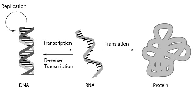
Figure 3.5. The “central dogma” of molecular biology. DNA is replicated during cell division. Information in DNA can also be transcribed into RNA, and, in some cases, the reverse can occur — information in RNA can be reverse transcribed into DNA. The information in RNA is translated into protein.

In the decades following the discovery of the central dogma, specific details have been added to it. For example, tiny cellular machines synthesize a complementary copy of RNA on the DNA template. These machines recognize specific sequences in DNA, directing them where to start synthesizing the RNA (Figure 3.6). Base pairing between DNA and RNA controls the sequence of the RNA molecule during RNA synthesis. Since RNA is virtually identical to DNA, except for an extra oxygen atom, the same chemical principles holding the DNA double helix together are what makes the DNA-RNA pairing possible. Thus, once the DNA is unzipped, RNA base pairs with DNA as well as — if not better than — another DNA molecule does (Figure 3.6).

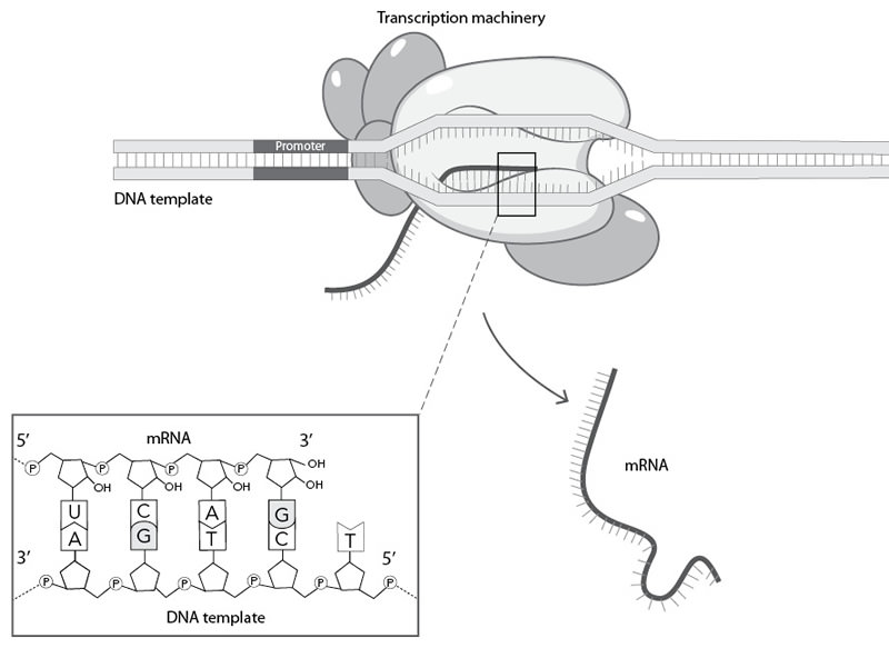
Figure 3.6. The process of transcription. Tiny cellular machines (symbolized by shaded ovals and other oblong shapes) recognize specific sequences in DNA (for example, a section of DNA, here labeled as a “promoter”). These machines then synthesize a complementary copy of RNA on the DNA template. Base pairing between DNA and RNA controls the sequence of the RNA molecule during RNA synthesis.

As the tiny reading and copying machine finishes synthesizing the protein-coding RNA, the DNA is re-zipped. The messenger RNA (RNA that codes for protein sequences) moves to another part of the cell where it encounters a translation machine called the ribosome (Figure 3.7). RNA-based adaptors (Crick’s hypothesized intermediates were finally discovered) translate the message into an amino acid sequence (Figure 3.7). Again, base pairing between the messenger RNA and the adaptor RNA (called transfer RNA or tRNA) makes the translation process possible (Figure 3.7). Each adaptor is chemically attached to a single amino acid (Figure 3.7). Because the adaptors match three base pairs at a time, the RNA code for protein is triplet in nature (Figure 3.7). As the ribosome reads through the messenger RNA molecule, the amino acids on each adaptor are taken off and attached to the growing protein chain (Figure 3.7). Once the final amino acid is attached, the ribosome structure dissociates, and the protein chain breaks free (Figure 3.7).12

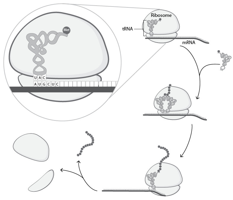
Figure 3.7. The process of translation. RNA that codes for protein sequences encounters a translation machine (the ribosome). RNA-based adaptors (tRNAs) translate the message into an amino acid sequence via base pairing between the messenger RNA and the tRNA. Each adaptor is chemically attached to a single amino acid (symbolized as a small circle). Because the adaptors match three base pairs at a time, the RNA code for protein is triplet in nature. As the ribosome reads through the messenger RNA molecule, the amino acids on each adaptor are taken off and attached to the growing protein chain, one amino acid at a time (because of space constraints, this diagram skips several of the individual amino acid attachment steps). Once the final amino acid is attached, the ribosome structure dissociates, and the protein chain breaks free.

Together, these discoveries uncovered an unprecedented role for DNA in the cell. By our analogy to the construction of a building, we’ve discovered that the encoded products of DNA, proteins, are multi-taskers. They transform energy, manufacture parts from raw materials, and act as the tools of the cell. By virtue of the fact that DNA codes for protein, we can see that DNA acts, at least in part, as the blueprint of the cell. Yet, extending our analogies even further, DNA isn’t a normal blueprint. It doesn’t just code for the structure of a creature. It also contains the information for the power plants, factories, and tool shops as well.

These discoveries also shed new light on Mendel’s observations from the preceding century. Prior to the 1950s, Mendel’s unit factors had been renamed genes. We now had a physical basis for understanding what unit factors — genes — actually were. They represented sections of DNA that coded for a protein, which performed some detectable function in the cell (Figure 3.8).

The origin of traits now seemed to be just a matter of understanding the origin of genes.

* * * *

The solution to the DNA-protein code took the scientific community one step closer to understanding how DNA controlled development. At the same time, other experimental results seemingly nullified this progress. Because the central dogma of molecular biology was cleverly solved without the knowledge of DNA sequences, the discovery of these sequences would represent a curious test of what was commonly accepted.

Even without actual DNA sequences, in the early 1950s indirect methods of DNA quantitation were disclosing an unsettling find. In these experiments, an investigator isolated cells from a species, estimated the number of cells in the sample under a microscope, and then chemically quantified the amount of DNA present. Dividing the amount of DNA by the number of cells yielded an estimate of the DNA per cell in a species.

Figure 3.8. Working definition of a gene. Mendel’s unit factors were eventually connected to genes — sections of DNA that coded for a protein, which performed some detectable function in the cell. Some genes are divided into protein-coding sections (“exons”) and non-protein-coding sections (“introns”). Introns are normally removed before the RNA sequence of a gene is translated by the ribosome.

In these experiments, you might expect simple creatures to have less DNA than more complex ones. Yet humans had the same amount of DNA per cell as a rat — and only slightly more than turtles and snakes. Among species without a backbone (e.g., invertebrates), sea urchins had roughly 6 times less DNA than humans, and snails only about 10 times less. Going the other direction on the DNA scale, some amphibians had 10 times more DNA than humans. Lungfish had nearly 20 times as much!13 If DNA was the blueprint of life, the amount of blueprint didn’t have a clear relationship with the amount and complexity of the creature to be built.

By the late 1960s and 1970s, the first complete DNA sequences — the genome — from various species were trickling in.14 The smallest genomes were solved first — the genomes of viruses. As might be expected from the central dogma, most of the DNA sequence in these genomes coded for proteins.

The first human sequences were from an unusual location. As we alluded to in a previous chapter, most of our DNA is contained in 46 chromosomes. But not all of it. In terms of physical location, these chromosomes reside in the subcellular compartment termed the nucleus (Figure 3.9). In the 1960s, DNA was detected elsewhere — in a different subcellular compartment termed the mitochondria.

With respect to the energy transformation functions we discussed earlier, mitochondria are the major sites (Figure 3.9). They contain numerous proteins involved in breaking down nutrients and coupling this to synthesis of ATP. Perhaps not surprisingly, then, when human mitochondrial DNA was sequenced in 1981,15 investigators discovered that it was chock-full of DNA sequences that coded for energy transformation proteins. It didn’t code for all the proteins that reside in mitochondria. But it was tightly packed with genes.

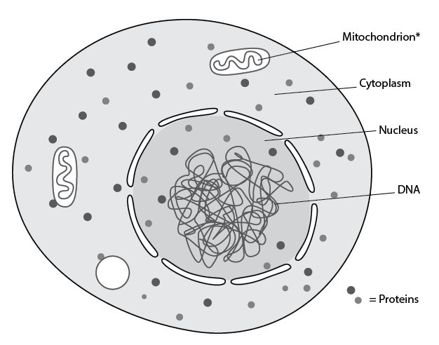
Figure 3.9. Location of DNA in the cell. The primary repository of DNA in the cell is the nucleus. *However, DNA is also found in another subcellular compartment, the mitochondria.

For the next several years, the main genomes that were cracked were from more viruses. The size of the sequenced genomes increased with time — from the 5,000 bases of the bacteriophage phi X174 genome in 1977 to the 237,000 base pair genome of the human cytomegalovirus in 1991. The evidence supporting the general expectations of the central dogma increased as well. The human cytomegalovirus genome was full of genes.

By now, the DNA sequences of the large animal genomes appeared within reach. In fact, in the late 1980s, discussions had already begun on whether the human genome should be formally tackled. Wisely, investigators planned a step-wise approach, choosing first to sequence genomes from key research organisms of increasing genome size. By targeting a bacterium, a yeast, a worm, and a fly, this approach would elucidate the genetics of a broad sampling of life. It would also allow DNA sequencing protocols to be optimized for the monumental task of sequencing the human genome.

Ironically, the first of these sequences to be published was not the smallest. In 1996, the 12 million base pair sequence of the single-celled baker’s yeast (Saccharomyces cerevisiae) appeared.16 The 4.6 million base pair genome of the common bacterium Escherichia coli (E. coli) followed in 1997.17 Nevertheless, both of these genomes still generally followed the expectations of the central dogma — they were packed with protein-coding genes.

By 1998, the first animal genome sequence appeared. At 97 million base pairs, the genome of the roundworm, Caenorhabditis elegans, represented one of the largest genome sequences uncovered to date. However, unlike the genomes of viruses and single-celled creatures, only around 27% of the Caenorhabditis elegans genome coded for proteins.18

What was the other 73% doing?

In 2000, the fruit fly (Drosophila melanogaster) genome of 120 million base pairs was published. It appeared to contain only about 13,600 genes.19 In contrast, the E. coli genome contained 3-fold fewer genes (4,288) — but was 26 times smaller (4.6 million base pairs). Fruit flies followed the pattern of rapidly increasing genome size and slowly increasing gene number.

In 2001, when the 3 billion base pair human genome20 was finally elucidated, only about 20,000–30,000 genes were found — roughly twice as many as the fruit fly. Furthermore, these genes represented only 1.5% of the human genome. Again, vast stretches of DNA didn’t fit the expectations of the central dogma.

In 2002, the mouse genome sequence was obtained. Like the human sequence, it was billions of base pairs long. Yet it contained few genes for its size — roughly the same number as the human genome.21 In other words, much of the mouse genome did not code for protein.

What was this non-coding DNA doing?

In the modern era of molecular biology, one way to test the function of a DNA sequence is by removing it — or, in molecular biology parlance, knocking it out. The initial experiments were done on a small scale. For example, gene deserts are long stretches of DNA without gene sequences. Over 2 million base pairs (i.e., a small fraction of the mouse genome) of a gene desert region were experimentally removed from the mouse genome, yet, in the parameters that the investigators measured, the mice were normal.22

If DNA was the blueprint for a creature, why did most of the blueprint in these multicellular creatures seem to not represent instructions for tools, power plants, and factories? In other words, if the code for a species’ morphology was hidden in DNA, why did the overwhelming majority of the sequence do something other than encode proteins? What was all this non-protein-coding DNA doing?

* * * *

Genome sequences revealed additional puzzles — at the level of genes themselves. If the relationship between genes and traits was as simple as the central dogma implied, then the results of gene mutation experiments would have been unremarkable and predictable. For example, each gene knockout would have resulted in an altered trait. In contrast, laboratory tests revealed a diversity of results — that spanned a wide spectrum of outcomes.

For instance, mutant fruit flies had been familiar to geneticists for a century. Long before DNA was established as the physical basis for heredity, heritable changes to the appearance of fruit flies had been documented and studied. One of the most dramatic mutants results in flies with legs protruding from the place where antenna normally attach (Figure 3.10). In other words, these mutant hox genes appeared to control the development of multiple traits.

Figure 3.10. Antennapedia mutation in fruit flies. In contrast to normal flies, Antennapedia mutant flies possess legs where antenna normally occur.

At the DNA level, when the sequence for several of these types of mutants was obtained, it differed from the sequence in non-mutant flies.23 The mutant DNA affected the activity of a protein that bound to DNA. This protein controlled the transcription, not of single genes, but whole batteries of genes. In general, it’s as if these hox genes sit near the top of a molecular circuit. When the molecular switch is flipped — when the Hox proteins bind DNA — they regulate the expression of an entire program of development.24 For example, the program for making a leg or an antenna.

The relationship between genes and traits was not as simple as it first appeared.

Other mutant genes had much less dramatic effects. For example, unlike fruit flies, mice often have, not one, but several copies of a gene in their genome. Where fruit flies might have one particular type of DNA binding gene, mice have several different versions of it (Figure 3.11 — hox genes).

This asymmetric relationship uncovered a perplexing pattern in mammals. Take the cell division cycle genes as a representative example. Since progression from a single cell to an adult mouse involves massive amounts of cell division, organisms must carefully regulate the process. (Cancer is an example of the process gone awry.) Not surprisingly, the mouse genome contains genes involved in controlling the cell division cycle. One particular type of regulatory protein is encoded by the cyclin D gene. Consistent with the pattern we observed with hox genes, mice possess three different versions of the cyclin D gene in their genomes—cyclin D1, cyclin D2, and cyclin D3.

Knocking out the cyclin D1, cyclin D2, or cyclin D3 genes individually produces little effect.25 If mice lack one of these individual genes, only a few tissues are effected; in other words, knocking out each of these does not result in embryonic lethality. For such a fundamental process as cell division, this result is very surprising. You might predict each of these proteins to be essential for life. Instead, only the simultaneous removal of all three cyclin D genes from the mouse genome results in embryonic lethality.26

Figure 3.11. Apparent genetic redundancy in more complex species. Similar genes can be found in fruit flies and mice. However, where fruit flies might have only one version of a particular gene — in this case a hox gene — mice might have four versions. Technically, because chromosomes come in pairs, fruit flies have two copies (one on each chromosome) of a gene, and mice have eight. But a 1:4 relationship (a “haploid” state) is shown for simplicity.

In other words, in our fruit fly example, some genes appeared to control multiple traits (hox genes). In contrast, in mice, some genes appeared to control very little — some genes appeared to be redundant.

When hundreds of genes were examined individually in mice, similar discoveries were made. Of mouse genes that have been knocked out individually, only around 40% are essential for mouse life.27

In other words, even when we restrict our focus to genes, the majority of mouse genes behave like non-protein-coding DNA — they sit in the genome, but appear to have no function.

These conclusions were not limited to mammals. Because of the smaller size and faster reproductive times in yeast and roundworms, more comprehensive tests of gene function were performed in these species. In yeast, over 6,000 genes were knocked out or inhibited — nearly the entire gene set.28 Eighty-six percent of roundworm genes have been tested in a similar way.29 In both cases, a small fraction of the total gene set was required for life. Thus, across animal and fungal kingdoms (i.e., one of the highest categories of biological classification), gene sequences behaved in odd and inexplicable ways.

* * * *

The resolution of these paradoxes arose from several cleverly designed experiments. For example, in all of the experiments on genome function that we discussed so far, the setting was the uniform conditions of the laboratory. In the wild, species face a diversity of conditions that are not present in the lab. This fact raised the possibility that the initial findings on genome function were an artifact of the laboratory setting.

In yeast, this hypothesis can be tested fairly easily. Since yeast are single-celled organisms, they can be grown in a wide variety of conditions, yet still be contained in a small physical space. One research team created over 1,000 different conditions. Then they repeated the screen for yeast gene function. Under these new experimental conditions, nearly every gene knockout resulted in defects under at least one condition.30

Another artifact of typical laboratory experiments is the narrow outcomes that investigators typically score. For example, in the initial comprehensive tests of roundworm gene function, the researchers recorded only whether the worms lived or died. Viability and lethality are very dramatic outcomes to test. (They also represent the simplest outcomes to test.) In contrast, in the wild, creatures fulfill many more functions than just survival. They must eat, grow, and reproduce, among other things. Conversely, a group of investigators repeated tests of gene function, but looked for more subtle, non-lethal effects of interfering with gene function. The majority of experimentally inhibited roundworm genes resulted in non-lethal defects.31

In light of these results in two very different creatures — creatures in different kingdoms, no less — we can revisit our initial conclusions in mice. With multiple organ systems and cell types, and with much longer lifespans than either yeast or roundworms, mice present a world of experimental conditions to test and a world of outcomes to score. Current methodologies barely scratch the surface in testing all of these. In short, in mice, the necessary, comprehensive, and labor-intensive experiments on genome function have not yet been performed. Until they are, it would be inappropriate to conclude that most genes — even most DNA — have little function.

In the meantime, one way to find a preliminary answer on the function of DNA sequences is via biochemical testing (i.e., tests that look for signatures of biochemical activity). These types of experiments are much easier to perform than genetic knock out experiments. Perhaps not surprisingly then, biochemical analyses have been done for nearly every base pair in the fruit fly,32 roundworm,33 mouse,34 and human35 genomes.

The trajectory of these experiments points toward pervasive, genome-wide function, including in the gene desert regions. In humans, preliminary biochemical evidence for function has been found for 80% of the base pairs in the human genome. Since protein-coding genes represent less than 2% of the total genome, a significant chunk of the 80% must represent gene desert regions.

But is this biochemical evidence relevant? Does a biochemical signature in a laboratory experiment have any bearing on how DNA might function in the wild? The history of these experiments suggests an answer.

For example, the first attempts to test the function of human DNA sequences in the laboratory were small. Only 1% of the total human DNA sequence was tested initially.36 Had the results been largely negative, you might have predicted the end of this project, termed the ENCODE project. Instead, the results were so promising that they prompted a test of the remaining 99% of the human genome.

In 2012, the results of the genome-wide study were published.37 These studies were the ones claiming evidence for function in around 80% of the human genome.38 One of the ENCODE project researchers speculated that, eventually, evidence would accumulate for function in nearly 100% of the human genome.39

This expectation is plausible for at least two reasons. First, when DNA sequences are plotted against organismal complexity, only a subsection of the genome shows a good positive correlation. Surprisingly, the protein-coding DNA is not a good predictor of biological complexity. Instead, non-protein-coding DNA tracks much better.40 This correlation implies that organismal complexity is encoded in the non-protein-coding section of the genome — which implies that this part of the genome is functional.

Second, despite the genomic comprehensiveness of the ENCODE project, it was biologically shallow. Consider: DNA is the instruction manual for building an organism, especially the traits that define each species. In creatures like mammals, these traits are generally absent at conception but present at birth. Therefore, from a purely theoretical perspective, much of the genome is likely used between conception and birth. Then, after birth, it might never be called upon again. The ENCODE project sampled hardly any of these conception-to-birth windows. I wouldn’t be surprised if the evidence for function sharply increases as investigators sample a greater diversity of cell types, of tissues, and of temporal windows of biological development.

Thus, when examined historically, the evidence for genome-wide function is gaining strength.

Together, these experiments suggested that the majority — if not the vast majority — of gene and non-genic DNA sequences were functional. The function might not be essential for life. But the genome appears to contain enormous amounts of information that act in ways yet to be fully explored.

* * * *

What specifically might non-protein-coding DNA be doing during development? Our analogy to construction sites for buildings suggests an answer. Consider the elements of the construction process that we’ve discussed: We’ve explored the need for transformed energy, manufactured materials, powered tools, and a blueprint. Now consider what’s missing: On their own, these four elements won’t automatically produce a skyscraper — or even a woodshed.

Why not?

Let’s derive the answer by comparing the construction site for a skyscraper to that for a woodshed. The major difference between these sites is not at the level of tools, power sources, or manufactured parts. To be sure, the former would require a slightly different set of tools than the latter. Also, steel beams and air conditioning units would be required in the former, and not the latter. But hammers, saws, screwdrivers, and other common tools would be present at both. Wood, nails, screws, and other common materials would be found in both places. In other words, the biggest differences between the sites would not be in the types of tools and materials present. It would be in the manner in which these tools and materials are used — in the timing and location of their application.

This difference is not borne out exclusively in the blueprint. A piece of paper doesn’t automatically result in the correct timing and location of the tools and materials. Rather, for these critical parts of the process to result in meaningful activity, a foreman must interpret the blueprint, coordinate the activity of worker crews, and ensure that the blueprint is correctly followed and enforced.

In our cellular construction project, what acts as the analogy for the foreman and human workers? In a sense, we’re asking what takes the place of the human mind. It’s one thing for the DNA to contain the instructions for how the pieces of the body are supposed to be put together. Enforcing and coordinating the necessary steps to make sure the pieces are put together in the correct temporal and spatial order is an entirely different task. In the cell, something must coordinate the temporal and spatial activity of the proteins — or a monster will result. What performs this task? And how does it do it? Does DNA get broken up and distributed among various cells?

Experiments by Sir John Gurdon in the 1950s and 1960s ruled out the latter. Gurdon was one of the first to perform cloning experiments. Other investigators before him had transplanted the nuclei of very early stage frog embryos into eggs in which the nuclei had been removed (i.e., enucleated eggs). Gurdon did the experiment with tadpole cells of an advanced developmental stage as sources of donor nuclei. After transplanting the nuclei into enucleated eggs and giving them a chance to develop, Gurdon found that he could recover fully-formed adults (Figure 3.12).41

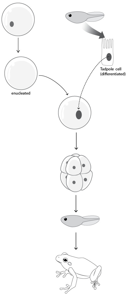
Figure 3.12. Gurdon’s successful frog cloning experiment. Sir John Gurdon transplanted the nuclei of tadpole cells of an advanced developmental stage into enucleated eggs (i.e., eggs in which the nuclei have been removed). After allowing these eggs with transplanted nuclei to develop, Gurdon found that he could recover fully-formed adults.

In the context of what we’ve already uncovered about DNA, Gurdon’s result suggested a curious conclusion. Since Gurdon used nuclei from highly developed cells as donors, he showed that development was reversible (at least, reversible at the level of single cells). In other words, since DNA is the stuff of heredity, the process of development appeared to not destroy the developmental potential of DNA. Furthermore, since nuclei — DNA — from advanced developmental stages still retained the capacity to recapitulate the developmental process, Gurdon’s results argued that the DNA sequence was the same in both embryonic and more developed cells.42 If development entailed shunting parts of the total DNA sequence — sections of each helix — into various cells, Gurdon’s results would never have occurred.

In the decades following, other experiments extended Gurdon’s conclusions. Cloning was successfully performed in mammals, and cloning was also achieved with fully developed cells from an adult.43 In addition, DNA sequencing studies confirmed the preservation of DNA during development. Despite obvious visible differences under the microscope among various cells of the body (Color Plate 16), the DNA in these cells was the same.

These results raised, again, the question of what substances in the cell substituted for a human foreman and workers. Clearly, since messenger RNA and protein levels differ among cells,44 something must be coordinating the timing and use of these substances. But what?

In the decades following the discovery of the central dogma, numerous additional discoveries have uncovered the means by which protein synthesis is regulated. The most obvious way to regulate the synthesis is by controlling when and where the RNA transcription machinery operates. These machines are, themselves, proteins. However, they bind to sequences that do not, themselves, code for protein.45

Sometimes the transcription process results in RNA that doesn’t get translated to protein. In fact, the DNA encoding these RNAs doesn’t look like protein-coding sequence. Instead, the sequence falls in the category of non-protein-coding DNA. The transcription of this non-protein-coding DNA produces RNAs that bind to DNA and affect the binding of transcription proteins.46

After transcription of messenger RNAs, regulation acts at each subsequent step of the process leading to protein synthesis. Eventually, messenger RNAs get degraded by the cell. Some RNAs are degraded quickly; others have longer lifespans.

If the messenger RNA survives long enough to reach the ribosome, further regulation modulates protein synthesis. Some messenger RNAs are translated quickly; others, more slowly.47 Like processes in the nucleus, some RNAs are synthesized, not for the purpose of being translated into protein, but for the purpose of binding to messenger RNAs and regulating the process of translation. In recent years, the number and types of newly discovered RNA molecules is expanding far beyond what anyone imagined.48

Together, the interactions among DNA, RNA, and protein coordinate the enforcement of the blueprint contained in DNA (Figure 3.13). In mind-numbing ways that we’re just beginning to uncover, the newly fertilized egg of a creature reads the instructions in DNA on how to transform energy, manufacture materials, connect them via powered tools in the right ways at the right locations and the right times, and then uses these instructions to assemble itself into a three-dimensional creature of enormous complexity. And it does so with extreme consistency and precision each time. As we have observed, the non-protein-coding DNA is an integral part of this process.49

* * * *

Despite the limitations of our current knowledge of function in the genome, the findings of molecular biology over the last several decades have uncovered a satisfying outline for the process of development. I used the word outline very deliberately. Even though the discoveries of the past several decades have uncovered a universe of activity inside cells, the process of development is one of the most baffling, mysterious, and unsolved puzzles in all of biology. Though great strides have been made since 1953, no one has discovered the step-by-step process by which an animal is built from a single cell. In fact, no one individual might ever possess this instruction manual. For one person to wrap their mind around all of the biological processes, steps, molecules, interactions, and developmental programs that are involved in development, they would need a lifetime of study — if not more. Consequently, possessing an outline of the process is a significant achievement.

Figure 3.13. The interactions among DNA, RNA, and protein control the process of development.

With this outline in hand, we can begin to sketch plausible hypotheses on how species acquire their traits each generation. For example, we can speculate on how zebras get their stripes. At the most basic level, proteins must surely be involved in the laying down of stripes in the zebra embryo. Since many proteins catalyze chemical synthesis and degradation steps, stripe production might be effected by proteins that catalyze the steps of the synthesis of a dark- or light-colored pigment.

At a deeper level, we can begin to formulate ideas on how this synthesis is regulated. If the pigment-synthesizing protein is allowed to perform catalysis in any and every cell all the time, the individual will be a solid color throughout. Conversely, if the protein is inhibited in any and every cell all the time, the individual will be a solid color throughout — but likely a different color than the individual with universally uninhibited protein activity.* Instead, if the creature prevents the protein (and, therefore, the pigment) from being made except in certain patches of skin cells, the creature will have a very distinct splotchy or patchy coat color.

You can imagine the result if activity is limited to certain stripes on the skin.50

In other creatures, speculating on the development of certain structures is more difficult. For example, unlike zebra stripes, the giraffe’s neck is much more than a surface decoration on an otherwise common anatomical pattern. Anatomically, like most mammals, giraffes have seven neck vertebrae.51 Yet their necks contain much more than bone; they also harbor muscles, blood vessels, and nerves. Consequently, producing longer necks requires changes, not only to bone, but also to muscle, blood vessel, and nervous system development. At the molecular level, major changes to the standard developmental pathway for vertebrae would be required to produce the giraffe’s signature structure.

In theory, these changes could take one of two forms. On the one hand, the standard developmental pathway for neck vertebrae production might involve changes to multiple proteins. Regulation might be altered for multiple individual proteins involved in blood vessel production, skeletal muscle production, and innervation. On the other hand, if master regulators of these developmental pathways exist, the regulation of these regulatory proteins (or, possibly, regulatory RNAs) might be changed.

A similar scenario exists in the case of the elephant’s trunk. Unlike the faces of so many other vertebrates, the development of the trunk involves the production of tens of thousands of additional muscles. Again, at the molecular level, major changes would be required to a standard developmental pathway — this time, the pathway for the development of the face. The regulation of multiple proteins might be each altered individually, or the regulation of a master regulator might be changed.

Thus, from relatively simple tasks like stripe production to comparatively challenging tasks like vertebrae elongation and trunk production, modern genetics is beginning to outline the steps by which these structures are built.

* * * *

Together, the observations of the last two chapters reveal how traits arise each generation. Despite the size and shape differences between sperm and egg, each carries the same number of chromosomes. Along these chromosomes, DNA double helices are tightly compacted. Along each double helix, the sequence of base pairs codes for RNA and proteins, and the interaction among these three molecules executes the developmental plan for each species.

The specific DNA differences among species explain specific aspects of the developmental process. For example, though visible traits are erased each generation, they are rebuilt in an extremely consistent manner. Consistent with this visible phenomenon, the vast majority of base pairs among individuals within a species are the same. For example, individual humans differ from one another at 0.1% to 0.6% of their base pairs.52 Similarly low percentages hold true in horses,53 donkeys,54 and dogs.55 Since 99% of the inherited DNA is the same each generation, it’s no wonder that the developmental process produces a consistent output each time.

This less-than-one-percent difference also explains the other side of the developmental coin. For example, though the output of the developmental process is extremely consistent each generation, offspring are not carbon copies of their parents. In other words, a small amount of change still happens each generation. Since DNA codes for traits, this change must be due to underlying DNA differences between offspring and parents. A less than 1% DNA difference fits this pattern of small changes each generation.

Extrapolating these processes backwards in time, we reach the answer to the bigger origins question. What we’ve observed thus far explains the origin of traits — but only over each generation. If we want to understand the origin of species, we must uncover the origin of the first traits. Since traits are ultimately encoded by DNA, the origin of species is a question of the origin of DNA differences within and between species. The answer to this question reveals whether a fish can spawn a spider — and whether it ever did.

In other words, by analogy to a jigsaw puzzle, the DNA differences among species represent the edge pieces to the puzzle — they set the hard limits and constraints on a potential explanation for the origin of species.

When Darwin wrote On the Origin of Species, he had no knowledge of the genetic processes that we explored in this chapter. DNA wasn’t recognized as the physical basis of heredity. No one had any idea how many DNA differences divided species. In fact, the DNA sequence of our own species wasn’t solved until 2001. Since our species is the best-studied multicellular species on the planet, you can appreciate how recently the genetics of other species have been elucidated.

In other words, the answer to the origin of species can be uncovered for the first time right now.