Chapter 6
Adaptive Filters
6.1 Introduction
Adaptive filters are used in situations where the characteristics or statistical properties of the signals involved are either unknown or time-varying. Typically, a nonadaptive FIR or IIR filter is designed with reference to particular signal characteristics. But if the signal characteristics encountered by such a filter are not those for which it was specifically designed, then its performance may be suboptimal. The coefficients of an adaptive filter are adjusted in such a way that its performance according to some measure improves with time and approaches optimum performance. Thus, an adaptive filter can be very useful either when there is uncertainty about the characteristics of a signal or when these characteristics are time-varying.
Adaptive systems have the potential to outperform nonadaptive systems. However, they are, by definition, nonlinear and more difficult to analyze than linear, time-invariant systems. This chapter is concerned with linear adaptive systems, that is, systems that, when adaptation is inhibited, have linear characteristics. More specifically, the filters considered here are adaptive FIR filters.
At the heart of the adaptive systems considered in this chapter is the structure shown in block diagram form in Figure 6.1.

Figure 6.1 Basic adaptive filter structure.
Its component parts are an adjustable filter, a mechanism for performance measurement (in this case, a comparator to measure the instantaneous error between adaptive filter output and desired output) and an adaptation mechanism or algorithm. In subsequent figures, the adaptation mechanism is incorporated into the adjustable filter block as shown in Figure 6.2
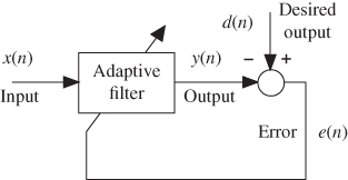
Figure 6.2 Simplified block diagram of basic adaptive filter structure.
It is conventional to refer to the coefficients of an adaptive FIR filter as weights, and the filter coefficients of the adaptive filters in several of the program examples in this chapter are stored in arrays using the identifier w rather than h as tended to be used for FIR filters in Chapter 3. The weights of the adaptive FIR filter are adjusted so as to minimize the mean squared value  of the error
  . The mean squared error
  is defined as the expected value, or hypothetical mean, of the square of the error, that is,
This quantity may also be interpreted as representing the variance, or power, of the error signal.
6.2 Adaptive Filter Configurations
Four basic configurations into which the adaptive filter structure of Figure 6.2 may be incorporated are commonly used. The differences between the configurations concern the derivation of the desired output signal  . Each configuration may be explained assuming that the adaptation mechanism will adjust the filter weights so as to minimize the mean squared value
  of the error signal
  but without the need to understand how the adaptation mechanism works.
6.2.1 Adaptive Prediction
In this configuration (Figure 6.3), a delayed version of the desired signal  is input to the adaptive filter, which predicts the current value of the desired signal
  . In doing this, the filter learns something about the characteristics of the signal
  and/or of the process that generated it. Adaptive prediction is used widely in signal encoding and noise reduction.

Figure 6.3 Basic adaptive filter structure configured for prediction.
6.2.2 System Identification or Direct Modeling
In this configuration (Figure 6.4), broadband noise  is input both to the adaptive filter and to an unknown plant or system. If adaptation is successful and the mean squared error is minimized (to zero in an idealized situation), then it follows that the outputs of both systems (in response to the same input signal) are similar and that the characteristics of the systems are equivalent. The adaptive filter has identified the unknown plant by taking on its characteristics. This configuration was introduced in Chapter 2 as a means of identifying or measuring the characteristics of an audio codec and was used again in some of the examples in Chapters 3 and 4. A common application of this configuration is echo cancellation in communication systems.

Figure 6.4 Basic adaptive filter structure configured for system identification.
6.2.3 Noise Cancellation
This configuration differs from the previous two in that while the mean squared error is minimized, it is not minimized to zero, even in the ideal case, and it is the error signal  rather than the adaptive filter output
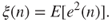
  that is the principal signal of interest. Consider the system illustrated in Figure 6.5. A primary sensor is positioned so as to pick up signal
  . However, this signal is corrupted by uncorrelated additive noise
  , that is, the primary sensor picks up signal
  . A second reference sensor is positioned so as to pick up noise from the same source as
  but without picking up signal
  . This noise signal is represented in Figure 6.5 as
  . Since they originate from the same source, it may be assumed that noise signals
  and
and  are strongly correlated. It is assumed here also that neither noise signal is correlated with signal
  . In practice, the reference sensor may pick up signal
  to some degree, and there may be some correlation between signal and noise, leading to a reduction in the performance of the noise cancellation system.
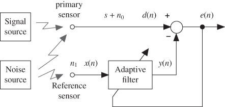
Figure 6.5 Basic adaptive filter structure configured for noise cancellation.
The noise cancellation system aims to subtract the additive noise  from the primary sensor output
  . The role of the adaptive filter is therefore to estimate, or derive,
  from
from  , and intuitively (since the two signals originate from the same source), this appears feasible.
An alternative representation of the situation described earlier, regarding the signals detected by the two sensors and the correlation between  and
and  , is shown in Figure 6.6. Here, it is emphasized that
  and
and  have taken different paths from the same noise source to the primary and reference sensors, respectively. Note the similarity between this and the system identification configuration shown in Figure 6.4. The mean squared error
  may be minimized if the adaptive filter is adjusted to have similar characteristics to the block shown between signals
  and
and  . In effect, the adaptive filter learns the difference in the paths between the noise source and the primary and reference sensors, represented in Figure 6.6 by the block labeled
  . The minimized error signal will, in this idealized situation, be equal to the signal
  , that is, a noise-free signal.

Figure 6.6 Alternative representation of basic adaptive filter structure configured for noise cancellation emphasizing the difference  in paths from a single noise source to primary and reference sensors.
6.2.4 Equalization
In this configuration (Figure 6.7), the adaptive filter is used to recover a delayed version of signal  from signal
  (formed by passing
  through an unknown plant or filter). The delay is included to allow for propagation of signals through the plant and adaptive filter. After successful adaptation, the adaptive filter takes on the inverse characteristics of the unknown filter, although there are limitations on the nature of the unknown plant for this to be achievable. Commonly, the unknown plant is a communication channel and
  is the signal being transmitted through that channel. It is natural at this point to ask why, if a delayed but unfiltered version of signal
  is available for use as the desired signal
  at the receiver, it is necessary to attempt to derive a delayed but unfiltered version of
  from signal
  . In general, a delayed version of
  is not available at the receiver, but for the purposes of adaptation over short periods of time, it is effectively made available by transmitting a predetermined sequence and using a copy of this stored at the receiver as the desired signal. In most cases, a pseudorandom, broadband signal is used for this purpose.

Figure 6.7 Basic adaptive filter structure configured for equalization.
6.3 Performance Function
Consider the block diagram representation of an FIR filter introduced in Chapter 3 and shown again in Figure 6.8.
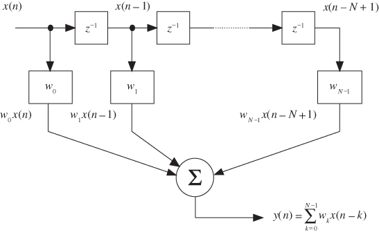
Figure 6.8 Block diagram representation of FIR filter.
In the following equations, the filter weights and the input samples stored in the FIR filter delay line at the  th sampling instant are represented as vectors
  and
and  , respectively, where

and

Hence, using vector notation, the filter output at the  th sample instant is given by

Instantaneous error is given by

and instantaneous squared error by

Mean squared error (expected value of squared error) is therefore given by

The expected value of a sum of variables is equal to the sum of the expected values of those variables. However, the expected value of a product of variables is the product of the expected values of the variables only if those variables are statistically independent. Signals  and
and  are generally not statistically independent. If the signals
  and
and  are statistically time-invariant, the expected values of the products
  and
and  are constants and hence
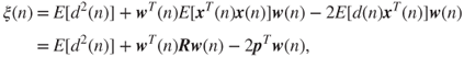
where the vector  of cross-correlation between input and desired output is defined as

and the input autocorrelation matrix  is defined as

The performance function, or surface,  is a quadratic function of
  and as such is referred to in the following equations as
  . Since it is a quadratic function of
  , it has one global minimum corresponding to
  . The optimum value of the weights,
  , may be found by equating the gradient of the performance surface to zero, that is,

and hence, in terms of the statistical quantities just described
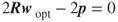
and hence,

In a practical, real-time application, solving Equation (6.13) may not be possible either because signal statistics are unavailable or simply because of the computational effort involved in inverting the input autocorrelation matrix  .
.
6.3.1 Visualizing the Performance Function
If there is just one weight in the adaptive filter, then the performance function will be a parabolic curve, as shown in Figure 6.9. If there are two weights, the performance function will be a three-dimensional surface, a paraboloid, and if there are more than two weights, then the performance function will be a hypersurface (i.e., difficult to visualize or to represent in a figure). In each case, the role of the adaptation mechanism is to adjust the filter coefficients to those values that correspond to a minimum in the performance function.

Figure 6.9 Performance function for single weight case.
6.4 Searching for the Minimum
An alternative to solving Equation (6.13) by matrix inversion is to search the performance function for  , starting with an arbitrary set of weight values and adjusting these at each sampling instant.
One way of doing this is to use the steepest descent algorithm. At each iteration (of the algorithm) in a discrete-time implementation, the weights are adjusted in the direction of the negative gradient of the performance function and by an amount proportional to the magnitude of the gradient, that is,
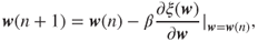
where  represents the value of the weights at the
  th iteration and
  is an arbitrary positive constant that determines the rate of adaptation. If
  is too large, then instability may ensue. If the statistics of the signals
  and
and  are known, then it is possible to set a quantitative upper limit on the value of
  , but in practice, it is usual to set
  equal to a very low value. One iteration of the steepest descent algorithm described by Equation (6.14) is illustrated for the case of a single weight in Figure 6.10.

Figure 6.10 Steepest descent algorithm illustrated for single weight case.
6.5 Least Mean Squares Algorithm
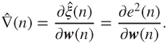
The steepest descent algorithm requires an estimate of the gradient  of the performance surface
  at each step. But since this depends on the statistics of the signals involved, it may be computationally expensive to obtain. The least mean squares (LMS) algorithm uses instantaneous error squared
  as an estimate of mean squared error
  and yields an estimated gradient

or
Equation (6.6) gave an expression for instantaneous squared error

Differentiating this with respect to  ,
,
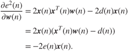
Hence, the steepest descent algorithm, using this gradient estimate, is
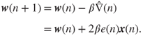
This is the LMS algorithm. Gradient estimate  is imperfect, and, therefore, the LMS adaptive process may be noisy. This is a further motivation for choosing a conservatively low value for
  .
.
The LMS algorithm is well established, computationally inexpensive, and, therefore, widely used. Other methods of adaptation include recursive least squares, which is more computationally expensive but converges faster, and normalized LMS, which takes explicit account of signal power. Given that in practice the choice of value for  is somewhat arbitrary, a number of simpler fixed step size variations are practicable although, somewhat counterintuitively, these variants may be computationally more expensive to implement using a digital signal processor with single-cycle multiply capability than the straightforward LMS algorithm.
6.5.1 LMS Variants
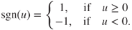
For the sign-error LMS algorithm, Equation (6.18) becomes

where  is the signum function
For the sign-data LMS algorithm, Equation (6.18) becomes

For the sign-sign LMS algorithm, Equation (6.18) becomes

which reduces to
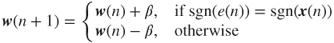
and which involves no multiplications.
6.5.2 Normalized LMS Algorithm
The rate of adaptation of the standard LMS algorithm is sensitive to the magnitude of the input signal  . This problem may be ameliorated by using the normalized LMS algorithm in which the adaptation rate
  in the LMS algorithm is replaced by

6.6 Programming Examples
The following program examples illustrate adaptive filtering using the LMS algorithm applied to an FIR filter.
This example implements the LMS algorithm as a C program. It illustrates the following steps for the adaptation process using the adaptive structure shown in Figure 6.2.
- Obtain new samples of the desired signal
 and the reference input to the adaptive filter
  .
. - Calculate the adaptive FIR filter output
 , applying Equation (6.4).
 - Calculate the instantaneous error
 by applying Equation (6.5).
 - Update the coefficient (weight) vector
 by applying the LMS algorithm (6.18).
 - Shift the contents of the adaptive filter delay line, containing previous input samples, by one.
- Repeat the adaptive process at the next sampling instant.
Program stm32f4_adaptive.c is shown in Listing 6.2. The desired signal is chosen to be  , and the input to the adaptive filter is chosen to be
  . The adaptation rate
  , filter order
  , and number of samples processed in the program are equal to 0.01, 21, and 60, respectively. The overall output is the adaptive filter output
  , which converges to the desired cosine signal
  .
.
Because the program does not use any real-time input or output, it is not necessary for it to call function stm32f4_wm5102_init(). Figure 6.11 shows plots of the desired output desired, adaptive filter output y_out, and error error, plotted using MATLAB® function stm32f4_plot_real() after the contents of those three arrays have been saved to files by typing
SAVE desired.dat <start address>, <start address + 0xF0>
SAVE y_out.dat <start address>, <start address + 0xF0>
SAVE error.dat <start address>, <start address + 0xF0>
in the Command window in the MDK-ARM debugger, where start address is the address of arrays desired, y_out, and error. Within 60 sampling instants, the filter output effectively converges to the desired cosine signal. Change the adaptation or convergence rate BETA to 0.02 and verify a faster rate of adaptation and convergence.

Figure 6.11 Plots of (a) desired output, (b) adaptive filter output, and (c) error generated using program stm32f4_adaptive.c and displayed using MATLAB function stm32f4_plot_real().
This example illustrates the use of the LMS algorithm to cancel an undesired sinusoidal noise signal. Listing 6.4 shows program tm4c123_adaptnoise_intr.c, which implements an adaptive FIR filter using the structure shown in Figure 6.5.
A desired sinusoid signal, of frequency SIGNAL_FREQ (2500 Hz), with an added (undesired) sinusoid signoise, of frequency NOISE_FREQ (1200 Hz), forms one of two inputs to the noise cancellation structure and represents the signal plus noise from the primary sensor in Figure 6.12. A sinusoid refnoise, with a frequency of NOISE_FREQ (1200 Hz), represents the reference noise signal in Figure 6.12 and is the input to an N-coefficient adaptive FIR filter. The signal refnoise is strongly correlated with the signal signoise but not with the desired signal. At each sampling instant, the output of the adaptive FIR filter is calculated, its N weights are updated, and the contents of the delay line x are shifted. The error signal is the overall desired output of the adaptive structure. It comprises the desired signal and additive noise from the primary sensor (signal + signoise) from which the adaptive filter output yn has been subtracted. The input signals used in this example are generated within the program and both the input signal signal + signoise and the output signal error are output via the AIC3104 codec on right and left channels, respectively.

Figure 6.12 Block diagram representation of program tm4c213_adaptnoise_intr.c.
Build and run the program and verify the following output result. The undesired 1200-Hz sinusoidal component of the output signal (error) is gradually reduced (canceled), while the desired 2500-Hz signal remains. A faster rate of adaptation can be observed by using a larger value of beta. However, if beta is too large, the adaptation process may become unstable. Program tm4c213_adaptnoise_intr.c demonstrates real-time adjustments to the coefficients of an FIR filter. The program makes use of CMSIS DSP library functions arm_sin_f32() and arm_cos_f32() in order to compute signal and noise signal values. Standard functions sin() and cos() would be computationally too expensive to use in real time. The adaptive FIR filter is implemented straightforwardly using program statements
  yn = 0;                 // compute adaptive filter output
  for (i = 0; i < N; i++)
    yn += (w[i] * x[i]);
  error = signal + signoise - yn;  // compute error
  for (i = N-1; i >= 0; i--)       // update weights
  {                                // and delay line
    dummy = BETA*error;
    dummy = dummy*x[i];
    w[i] = w[i] + dummy;
    x[i] = x[i-1];
  }
in which the entire contents of the filter delay line x are shifted at each sampling instant. Program tm4c123_adaptnoise_CMSIS_intr.c shown in Listing 6.5 makes use of the more computationally efficient CMSIS DSP library function arm_lms_f32().
6.6.1 Using CMSIS DSP Function arm_lms_f32()
In order to implement an adaptive FIR filter using CMSIS DSP library function arm_lms_f32(), as in the previous example, the following variables must be declared.
- A structure of type
arm_lms_instance_f32 - A floating-point state variable array
firStateF32 - A floating-point array of filter coefficients
firCoeffs32.
The arm_lms_instance_f32 structure comprises an integer value equal to the number of coefficients, N used by the filter, a floating-point value equal to the learning rate BETA, and pointers to the array of N floating-point filter coefficients and to the N + BLOCKSIZE - 1 floating-point state variable array. The state variable array contains current and previous values of the input to the filter. Before calling function arm_lms_f32(), the structure is initialized using function arm_lms_init_f32(). This assigns values to the elements of the structure and initializes the contents of the state variable array to zero. Function arm_lms_init_f32() does not allocate memory for the filter coefficient or state variable arrays. They must be declared separately. Function arm_lms_init_f32() does not initialize or alter the contents of the filter coefficient array.
Subsequently, function arm_lms_f32() may be called, passing to it pointers to the arm_lms_instance_f32 structure and to floating-point arrays of input samples, output samples, desired output samples, and error samples. Each of these arrays contains BLOCKSIZE samples. Each call to function arm_lms_f32() processes BLOCKSIZE samples, and although it is possible to set BLOCKSIZE to one, the function is optimized according to the architecture of the ARM Cortex-M4 to operate on at least four samples per call. More details of function arm_lms_f32() can be found in the CMSIS documentation [1].
This example extends the previous one to cancel an undesired noise signal using external inputs. Program stm32f4_noise_cancellation_CMSIS_dma.c, shown in Listing 6.7, requires two external inputs, a desired signal, and a reference noise signal to be input to left and right channels of LINE IN, respectively. A stereo 3.5-mm jack plug to dual RCA jack plug cable is useful for implementing this example using two different signal sources. Alternatively, a test input signal is provided in file speechnoise.wav. This may be played through a PC sound card and input to the audio card via a stereo 3.5 mm jack plug to 3.5 mm jack plug cable. speechnoise.wav comprises pseudorandom noise on the left channel and speech on the right channel.
Figure 6.13 shows the program in block diagram. Within the program, a primary noise signal, correlated to the reference noise signal input on the left channel, is formed by passing the reference noise through an IIR filter. The primary noise signal is added to the desired signal (speech) input on the right channel.

Figure 6.13 Block diagram representation of program tm4c123_noise_cancellation_intr.c.
Build and run the program and test it using file speechnoise.wav. As adaptation takes place, the output on the left channel of LINE OUT should gradually change from speech plus noise to speech only. You may need to adjust the volume at which you play the file speechnoise.wav. If the input signals are too quiet, then adaptation may be very slow. This is an example of the disadvantage of the LMS algorithm versus the NLMS algorithm. After adaptation has taken place, the 32 coefficients of the adaptive FIR filter, firCoeffs32, may be saved to a data file by typing
SAVE <filename> <start address>, <end address>in the Command window of the MDK-ARM debugger, where start address is the address of array firCoeffs32 and end address is equal to start address + 0x80, and plotted using MATLAB function stm32f4_logfft(). This should reveal the time- and frequency-domain characteristics of the IIR filter implemented by the program, as identified by the adaptive filter and as shown in Figure 6.14.

Figure 6.14 Impulse response and magnitude frequency response of IIR filter identified by the adaptive filter in program tm4c123_noise_cancellation_intr.c and plotted using MATLAB function tm4c123_logfft().
Listing 6.9 shows program tm4c123_adaptIDFIR_CMSIS_intr.c, which uses an adaptive FIR filter to identify an unknown system. A block diagram of the system implemented in this example is shown in Figure 6.15. The unknown system to be identified is a 55-coefficient FIR band-pass filter centered at 2000 Hz. The coefficients of this fixed FIR filter are read from header file bp55.h, previously used in Example 3.23. A 60-coefficient adaptive FIR filter is used to identify the fixed (unknown) FIR band-pass filter.

Figure 6.15 Block diagram representation of program tm4c123_adaptIDFIR_CMSIS_intr.c.
A pseudorandom binary noise sequence, generated within the program, is input to both the fixed (unknown) and the adaptive FIR filters and an error signal formed from their outputs. The adaptation process seeks to minimize the variance of that error signal. It is important to use wideband noise as an input signal in order to identify the characteristics of the unknown system over the entire frequency range from zero to half the sampling frequency.
Build, load, and run the program. The blue user pushbutton on the Discovery may be used to toggle the output between y_fir (the output from the fixed (unknown) FIR filter) and y_lms (the output from the adaptive FIR filter) as the signal written to the right channel of LINE OUT on the audio card. error (the error signal) is always written to the left channel of LINE OUT. Verify that the output of the adaptive FIR filter (y_lms) converges to bandlimited noise similar in frequency content to the output of the fixed FIR filter (y_fir) and that the variance of the error signal (error) gradually diminishes as adaptation takes place.
Edit the program to include the coefficient file bs55.h (in place of bp55.h), which implements a 55-coefficient FIR band-stop filter centered at 2 kHz. Rebuild and run the program and verify that, after adaptation has taken place, the output of the adaptive FIR filter is almost identical to that of the FIR band-stop filter. Figure 6.16 shows the output of the program while adaptation is taking place. The upper time-domain trace shows the output of the adaptive FIR filter, the lower time-domain trace shows the error signal, and the magnitude of the FFT of the output of the adaptive FIR filter is shown below them. Increase (or decrease) the value of beta by a factor of 10 to observe a faster (or slower) rate of convergence. Change the number of weights (coefficients) from 60 to 40 and verify a slight degradation in the identification process. You can examine the adaptive filter coefficients stored in array firCoeffs32 in this example by saving them to data file and using the MATLAB function stm32f4_logfft() to plot them in the time and frequency domains.

Figure 6.16 Output from program stm32f4_adaptIDFIR_CMSIS_intr.c using coefficient header file bs55.h viewed using Rigol DS1052E oscilloscope.
In this example, program stm32f4_adaptIDFIR_CMSIS_intr.c has been modified slightly in order to create program stm32f4_adaptIDFIR_init_intr.c. This program initializes the weights, firCoeffs32, of the adaptive FIR filter using the coefficients of an FIR band-pass filter centered at 3 kHz, rather than initializing the weights to zero. Both sets of filter coefficients (adaptive and fixed) are read from file adaptIDFIR_CMSIS_init_coeffs.h. Build, load, and run the program. Initially, the frequency content of the output of the adaptive FIR filter is centered at 3 kHz. Then, gradually, as the adaptive filter identifies the fixed (unknown) FIR band-pass filter, its output changes to bandlimited noise centered on frequency 2 kHz. The adaptation process is illustrated in Figure 6.17, which shows the frequency content of the output of the adaptive filter at different stages in the adaptation process.

Figure 6.17 Output from adaptive filter in program tm4c123_adaptIDFIR_CMSIS_init_intr.c.
As in most of the example programs in this chapter, the rate of adaptation has been set very low.
An adaptive FIR filter can be used to identify the characteristics not only of other FIR filters but also of IIR filters (provided that the substantial part of the IIR filter impulse response is shorter than that possible using the adaptive FIR filter). Program tm4c123_iirsosadapt_CMSIS_intr.c, shown in Listing 6.12 combines programs tm4c123_iirsos_intr.c (Example 4.2) and tm4c123_adaptIDFIR_CMSIS_intr.c in order to illustrate this (Figure 6.18). The IIR filter coefficients used are those of a fourth-order low-pass elliptic filter (see Example 4.9) and are read from file elliptic.h. Build and run the program and verify that the adaptive filter converges to a state in which the frequency content of its output matches that of the (unknown) IIR filter. Listening to the decaying error signal output on the left channel of LINE OUT on the audio booster pack gives an indication of the progress of the adaptation process. Figures 6.19 and 6.20 show the output of the adaptive filter (displayed using the FFT function of a Rigol DS1052E oscilloscope) and the magnitude FFT of the coefficients (weights) of the adaptive FIR filter saved to a data file and displayed using MATLAB function tm4c123_logfft(). The result of the adaptive system identification procedure is similar in form to that obtained by recording the impulse response of an elliptic low-pass filter using program tm4c123_iirsosdelta_intr.c in Example 4.10.
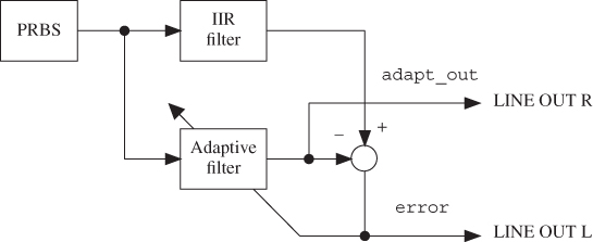
Figure 6.18 Block diagram representation of program tm4c123_iirsosadapt_CMSIS_intr.c.

Figure 6.19 Output from adaptive filter in program tm4c123_iirsosadapt_CMSIS_intr.c viewed using a Rigol DS1052E oscilloscope.

Figure 6.20 Adaptive filter coefficients from program tm4c123_iirsosadapt_CMSIS_intr.c plotted using MATLAB function tm4c123_logfft().
Program tm4c123_sysid_CMSIS_intr.c, introduced in Chapter 2, extends the previous examples to allow the identification of an external system, connected between the LINE OUT and LINE IN sockets of the audio booster pack. In Example 3.17, program tm4c123_sysid_CMSIS_intr.c was used to identify the characteristics of a moving average filter implemented using a second TM4C123 LaunchPad and audio booster pack. Alternatively, a purely analog system or a filter implemented using different DSP hardware can be connected between LINE OUT and LINE IN and its characteristics identified. Connect two systems as shown in Figure 6.21. Load and run tm4c123_iirsos_intr.c, including coefficient header file elliptic.h on the first. Run program tm4c123_sysid_CMSIS_intr.c on the second. Halt program tm4c123_sysid_CMSIS_intr.c after a few seconds and save the 256 adaptive filter coefficients firCoeffs32 to a data file. You can plot the saved coefficients using MATLAB function tm4c123_logfft(). Figure 6.22 shows typical results.

Figure 6.21 Connection diagram for program tm4c123_sysid_CMSIS_intr.c in Example 6.14.

Figure 6.22 Adaptive filter coefficients from program tm4c123_sysid_CMSIS_intr.c plotted using MATLAB function tm4c123_logfft()
A number of features of the plots shown in Figure 6.22 are worthy of comment. Compare the magnitude frequency response in Figure 6.22(b) with that in Figure 6.20(b). The characteristics of the codec reconstruction and antialiasing filters and of the ac coupling between codecs and jack sockets on both boards are included in the signal path identified by program tm4c123_sysid_CMSIS_intr.c in this example and are apparent in the roll-off of the magnitude frequency response at frequencies above 3800 Hz and below 100 Hz. There is no roll-off in Figure 6.20(b). Compare the impulse response in Figure 6.22(b) with that in Figure 6.20(b). Apart from its slightly different form, corresponding to the roll-off in its magnitude frequency response, there is an additional delay of approximately 12 ms.
Functionally, program tm4c123_sysid_CMSIS_dma.c (Listing 6.15) is similar to program tm4c123_sysid_CMSIS_intr.c. Both programs use an adaptive FIR filter, implemented using CMSIS DSP library function arm_lms_f32(), to identify the impulse response of a system connected between LINE OUT and LINE IN connections to the audio booster pack. However, program tm4c123_sysid_CMSIS_dma.c is more computationally efficient and can run at higher sampling rates. Because function arm_lms_f32() is optimized to process blocks of input data rather than just one sample at a time, it is appropriate to use DMA-based rather than interrupt-based i/o in this example. However, DMA-based i/o introduces an extra delay into the signal path identified, and this is evident in the examples of successfully adapted weights shown in Figure 6.23. In each case, the adaptive filter used 256 weights. The program has been run successfully using up to 512 weights at a sampling rate of 8 kHz on the TM4C123 LaunchPad with a processor clock rate of 84 MHz.
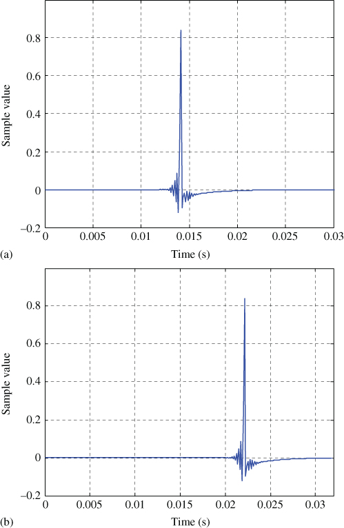
Figure 6.23 Adaptive filter coefficients from program tm4c123_sysid_CMSIS_dma.c plotted using MATLAB function tm4c123_logfft(). (a) BUFSIZE = 32 (b) BUFSIZE = 64.