Although regular hidden layers (we also call them fully connected layers) do the job of obtaining representations at certain levels, these representations might be able to help us differentiate between images of different classes. We need to extract richer and distinguishable representations that, for example, make a "9" a "9", a "4" a "4", or a cat a cat, a dog a dog. We resort to CNNs as variants of multi-layered neural networks which are biologically inspired by the human visual cortex. Basically, CNNs take inspiration from the following two neuroscience findings:
- The visual cortex has a complex system of neuronal cells that are sensitive to specific sub-regions of the visual field, called the receptive field. For instance, some cells respond only in the presence of vertical edges; some cells fire only when exposed to horizontal edges; and some react more strongly when shown edges of a certain orientation. The cells are organized together to produce the entire visual perception, while each individual cell is specialized in a specific component.
- Simple cells respond only when those edge-like patterns are presented within their receptive sub-regions. More complex cells are sensitive to larger sub-regions, and as a result, are less variant to the local position of those edge-like patterns in the entire visual field.
Similarly, CNNs classify images by first deriving low-level representations, local edges and curves, then by composing higher-level representations, overall shape and contour, through a series of low-level representations. CNNs are well suited to exploiting strong and unique features that differentiate between images.
In general, CNNs take in an image, pass it through a sequence of convolutional layers, non-linear layers, pooling layers and fully connected layers, and finally output the probabilities of each possible class. We now look at each type of layer individually, in detail.
The convolutional layer is the first layer in a CNN. It simulates the way neuronal cells respond to receptive fields by applying a convolutional operation to the input. To be specific, it computes the dot product between the weights of the convolutional layer and a small region they are connected to in the input layer. The small region is the receptive field, and the weights can be viewed as the values on a filter. As the filter slides from the beginning to the end of the input layer, the dot product between the weights and current receptive field is computed. A new layer called feature map is obtained after convolving over all sub-regions. Take a look at the following example:

Layer m has five nodes and the filter has three units [w1, w2, w3]. We compute the dot product between the filter and the first three nodes in layer m and obtain the first node in the feature map; then, we compute the dot product between the filter and the middle three nodes and generate the second node; finally, we obtain the third node resulting from the last three nodes in layer m.
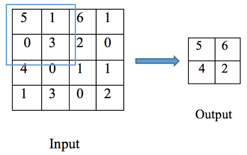
Another example that helps us better understand how the convolutional layer works on images is as follows:

A 3*3 filter is sliding around a 5*5 image from the top left sub-region to the bottom right. For every sub-region, the dot product is computed with the filter. A 3*3 feature map is generated as a result.
Convolutional layers are actually used to extract features, such as edges and curves. The output pixel in the feature map will be of high value, if the corresponding receptive field contains an edge or curve specified by the filter. For instance, in the preceding example, the filter portrays a backslash-shape diagonal edge, the receptive field in the blue rectangle contains a similar curve and hence, the highest intensity 3 (1*1 + 1* 1 + 1*1 = 3) is produced; however, the receptive field in the bottom left corner does not contain such a shape, which results in a pixel of value 1. The convolutional layer acts as a curve detector, mimicking the way our visual cells work.
Remember in the preceding case, we only applied one filter and generated one feature map, which indicates how well the shape in the input image resembles the curve represented in the filter. To achieve a richer representation of the data, we can employ more filters, such as horizontal, vertical curve, 30-degree, or right-angle shape, so that the hidden layer composed of feature maps can detect more patterns. Additionally, stacking many convolutional layers can produce higher-level representations, such as overall shape and contour. To ensure the strong spatially local patterns are caught, each filter in a layer is only responsive to the corresponding receptive fields. Chaining more layers results in larger receptive fields which capture more global patterns.
Right after each convolutional layer, we often apply a non-linear layer (also called activation layer, as we mentioned), in order to introduce non-linearity, obviously. This is because only linear operations (multiplication and addition) are conducted in the convolutional layer. And a neural network with only linear hidden layers would behave just like a single-layer perceptron, regardless of how many layers. Again, ReLu is the most popular candidate for the non-linear layer in deep neural networks.
Normally, after obtaining features via one or more pairs of convolutional layers and non-linear layers, we can use the output for classification, for example applying a softmax layer in our multiclass case. Let's do some math, suppose we apply 20 5*5 filters in the first convolutional layer, then the output of this layer will be of size 20 * (28 - 5 + 1) * (28 - 5 + 1) = 20 * 24 * 24 = 11520, which means the number of features as inputs for the next layer becomes 11,520 from 784; we then apply 50 5*5 filters in the second convolutional layer, the size of the output grows to 50 * 20 * (24 - 5 + 1) * (24 - 5 + 1) = 400,000, which is high-dimensional compared to our initial size of 784. We can see that the dimension increases dramatically with each convolutional layer before the softmax layer for classification. This can easily lead to overfitting, not to mention the large number of weights to be trained in the corresponding non-linear layer.
To address the dimension growth issue, we often employ a pooling layer (also called downsampling layer) after a pair of convolutional and non-linear layers. As its name implies, it aggregates statistics of features by sub-regions to generate much lower dimensional features. Typical pooling methods include max pooling and mean pooling, which take the max values and mean values over all non-overlapping sub-regions, respectively. For example, we apply a 2*2 max pooling filter on a 4*4 feature map and output a 2*2 one:
Besides reducing overfitting with lower dimensional output, the pooling layer aggregating statistics over regions has another advantage—translation invariant. It means the output does not change, if the input image undergoes a small amount of translation. For example, suppose we shift the input image to a couple of pixels left or right, up or down, as long as the highest pixels remain the same in sub-regions, the output of the max pooling layer is still the same. In another words, the prediction becomes less position-sensitive with pooling layers.
Putting these three types of convolutional-related layers together, along with fully connected layers, we can structure our CNN model as follows:

It starts with the first convolutional layer, ReLu non-linear layer and pooling layer. Here, we use 20 5*5 convolutional filters, and a 2*2 max pooling filter:
> # first convolution
> conv1 <- mx.symbol.Convolution(data=data, kernel=c(5,5),
num_filter=20)
> act1 <- mx.symbol.Activation(data=conv1, act_type="relu")
> pool1 <- mx.symbol.Pooling(data=act1, pool_type="max",
+ kernel=c(2,2), stride=c(2,2))
It follows with the second convolutional, ReLu non-linear and pooling layer, where 50 5*5 convolutional filters and a 2*2 max pooling filter are used:
> # second convolution
> conv2 <- mx.symbol.Convolution(data=pool1, kernel=c(5,5),
num_filter=50)
> act2 <- mx.symbol.Activation(data=conv2, act_type="relu")
> pool2 <- mx.symbol.Pooling(data=act2, pool_type="max",
+ kernel=c(2,2), stride=c(2,2))
Now that we extract rich representations of the input images by detecting edges, curves and shapes, we move on with the fully connected layers. But before doing so, we need to flatten the resulting feature maps from previous convolution layers:
> flatten <- mx.symbol.Flatten(data=pool2)
In the fully connected section, we apply two ReLu hidden layers with 500 and 10 units respectively:
> # first fully connected layer
> fc1 <- mx.symbol.FullyConnected(data=flatten, num_hidden=500)
> act3 <- mx.symbol.Activation(data=fc1, act_type="relu")
> # second fully connected layer
> fc2 <- mx.symbol.FullyConnected(data=act3, num_hidden=10)
Finally, the softmax layer producing outputs for 10 classes:
> # softmax output
> softmax <- mx.symbol.SoftmaxOutput(data=fc2, name="sm")
Now, the bone is constructed. Time to set a random seed and start training the model:
We need to first reshape the matrix, data_train.x into an array as required by the convolutional layer in MXNet:
> train.array <- data_train.x
> dim(train.array) <- c(28, 28, 1, ncol(data_train.x))
> mx.set.seed(42)
> model_cnn <- mx.model.FeedForward.create(softmax, X=train.array,
y=data_train.y, ctx=devices, num.round=30,
array.batch.size=100, learning.rate=0.05,
momentum=0.9, wd=0.00001,
eval.metric=mx.metric.accuracy,
epoch.end.callback=mx.callback.log.train.metric(100))
Start training with 1 devices
[1] Train-accuracy=0.306984126984127
[2] Train-accuracy=0.961898734177216
[3] Train-accuracy=0.981139240506331
[4] Train-accuracy=0.987151898734179
[5] Train-accuracy=0.990348101265825
[6] Train-accuracy=0.992689873417723
[7] Train-accuracy=0.994493670886077
[8] Train-accuracy=0.995822784810128
[9] Train-accuracy=0.995601265822786
[10] Train-accuracy=0.997246835443039
[11] Train-accuracy=0.997341772151899
[12] Train-accuracy=0.998006329113925
[13] Train-accuracy=0.997626582278482
[14] Train-accuracy=0.998069620253165
[15] Train-accuracy=0.998765822784811
[16] Train-accuracy=0.998449367088608
[17] Train-accuracy=0.998765822784811
[18] Train-accuracy=0.998955696202532
[19] Train-accuracy=0.999746835443038
[20] Train-accuracy=0.999841772151899
[21] Train-accuracy=0.999905063291139
[22] Train-accuracy=1
[23] Train-accuracy=1
[24] Train-accuracy=1
[25] Train-accuracy=1
[26] Train-accuracy=1
[27] Train-accuracy=1
[28] Train-accuracy=1
[29] Train-accuracy=1
[30] Train-accuracy=1
Besides those hyperparameters we used in the previous deep neural network model, we fit the CNN model with L2 regularization weight decay wd = 0.00001, which adds penalties for large weights in order to avoid overfitting.
Again, training of the CNN model is no different to other networks. Optimal weights are obtained through a backpropagation algorithm.
After the model is trained, let's see how it performs on the testing set. First, remember to conduct the same pre-processing on the test dataset:
> test.array <- data_test.x
> dim(test.array) <- c(28, 28, 1, ncol(data_test.x))
Predict the testing cases and evaluate the performance:
> prob_cnn <- predict(model_cnn, test.array)
> prediction_cnn <- max.col(t(prob_cnn)) - 1
> cm_cnn = table(data_test$label, prediction_cnn)
> cm_cnn
prediction_cnn
0 1 2 3 4 5 6 7 8 9
0 1051 0 1 0 0 1 1 0 2 0
1 0 1161 0 0 0 1 1 3 1 0
2 0 0 1014 4 0 0 0 7 0 0
3 0 0 2 1075 0 6 0 2 3 2
4 0 0 0 0 1000 0 4 2 2 7
5 1 0 0 4 0 923 3 0 3 3
6 3 0 0 0 0 0 1006 0 1 0
7 0 1 2 0 3 0 0 1129 1 0
8 3 3 1 1 2 5 1 0 1043 6
9 2 0 2 0 3 3 1 2 0 984
> accuracy_cnn = mean(prediction_cnn == data_test$label)
> accuracy_cnn
[1] 0.9893313
Our CNN model further boosts the accuracy to close to 99%!
We can also view the network structure by:
> graph.viz(model_cnn$symbol)
Let's do some more inspection to make sure we get things right. We start with the learning curving, for example the classification performance of the model on both the training set and testing set over the number of training iterations. In general, it is a good practice to plot the learning curve where we can visualize whether overfitting or underfitting issues occur:
> data_test.y <- data_test[,1]
> logger <- mx.metric.logger$new()
> model_cnn <- mx.model.FeedForward.create(softmax, X=train.array,
y=data_train.y,eval.data=list(data=test.array,
label=data_test.y), ctx=devices, num.round=30,
array.batch.size=100, learning.rate=0.05,
momentum=0.9, wd=0.00001,eval.metric=
mx.metric.accuracy, epoch.end.callback =
mx.callback.log.train.metric(1, logger))
Start training with 1 devices
[1] Train-accuracy=0.279936507936508
[1] Validation-accuracy=0.912857142857143
[2] Train-accuracy=0.959462025316456
[2] Validation-accuracy=0.973523809523809
[3] Train-accuracy=0.979841772151899
[3] Validation-accuracy=0.980666666666666
[4] Train-accuracy=0.986677215189875
[4] Validation-accuracy=0.983428571428571
[5] Train-accuracy=0.990822784810129
[5] Validation-accuracy=0.981809523809523
[6] Train-accuracy=0.992626582278482
[6] Validation-accuracy=0.983904761904761
[7] Train-accuracy=0.993322784810128
[7] Validation-accuracy=0.986
[8] Train-accuracy=0.995474683544305
[8] Validation-accuracy=0.987619047619047
[9] Train-accuracy=0.996487341772153
[9] Validation-accuracy=0.983904761904762
[10] Train-accuracy=0.995949367088608
[10] Validation-accuracy=0.984761904761904
[11] Train-accuracy=0.997310126582279
[11] Validation-accuracy=0.985142857142856
[12] Train-accuracy=0.997658227848102
[12] Validation-accuracy=0.986857142857142
[13] Train-accuracy=0.997848101265824
[13] Validation-accuracy=0.984095238095238
[14] Train-accuracy=0.998006329113924
[14] Validation-accuracy=0.985238095238094
[15] Train-accuracy=0.998607594936709
[15] Validation-accuracy=0.987619047619047
[16] Train-accuracy=0.99863924050633
[16] Validation-accuracy=0.987428571428571
[17] Train-accuracy=0.998987341772152
[17] Validation-accuracy=0.985142857142857
[18] Train-accuracy=0.998765822784811
[18] Validation-accuracy=0.986285714285713
[19] Train-accuracy=0.999240506329114
[19] Validation-accuracy=0.988761904761905
[20] Train-accuracy=0.999335443037975
[20] Validation-accuracy=0.98847619047619
[21] Train-accuracy=0.999841772151899
[21] Validation-accuracy=0.987809523809523
[22] Train-accuracy=0.99993670886076
[22] Validation-accuracy=0.990095238095237
[23] Train-accuracy=1
[23] Validation-accuracy=0.989999999999999
[24] Train-accuracy=1
[24] Validation-accuracy=0.989999999999999
[25] Train-accuracy=1
[25] Validation-accuracy=0.990190476190476
[26] Train-accuracy=1
[26] Validation-accuracy=0.990190476190476
[27] Train-accuracy=1
[27] Validation-accuracy=0.990095238095237
[28] Train-accuracy=1
[28] Validation-accuracy=0.990095238095237
[29] Train-accuracy=1
[29] Validation-accuracy=0.990095238095237
[30] Train-accuracy=1
[30] Validation-accuracy=0.990190476190475
We can get the performance on the training set after each round of training:
> logger$train
[1] 0.2799365 0.9594620 0.9798418 0.9866772 0.9908228 0.9926266 0.9933228 0.9954747 0.9964873 0.9959494 0.9973101
[12] 0.9976582 0.9978481 0.9980063 0.9986076 0.9986392 0.9989873 0.9987658 0.9992405 0.9993354 0.9998418 0.9999367
[23] 1.0000000 1.0000000 1.0000000 1.0000000 1.0000000 1.0000000 1.0000000 1.0000000
As well as the performance on the testing set after each round of training:
> logger$eval
[1] 0.9128571 0.9735238 0.9806667 0.9834286 0.9818095 0.9839048 0.9860000 0.9876190 0.9839048 0.9847619 0.9851429
[12] 0.9868571 0.9840952 0.9852381 0.9876190 0.9874286 0.9851429 0.9862857 0.9887619 0.9884762 0.9878095 0.9900952
[23] 0.9900000 0.9900000 0.9901905 0.9901905 0.9900952 0.9900952 0.9900952 0.9901905
The learning curve can be visualized by the following codes:
> plot(logger$train,type="l",col="red", ann=FALSE)
> lines(logger$eval,type="l", col="blue")
> title(main="Learning curve")
> title(xlab="Iterations")
> title(ylab="Accuary")
> legend(20, 0.5, c("training","testing"), cex=0.8,
col=c("red","blue"), pch=21:22, lty=1:2);
And we will get:

The learning curve indicates little chance of overfitting or underfitting.
Since the model works great, why don't we visualize the output of the convolutional layers of the trained model so that we can get a better understanding of CNNs. Let's use the first two samples in the testing set as an example. They are 1 and 0:
> par(mfrow=c(1,2))
> test_1 <- matrix(as.numeric(data_test[1,-1]), nrow = 28,
byrow = TRUE)
> image(rotate(test_1), col = grey.colors(255))
> test_2 <- matrix(as.numeric(data_test[2,-1]), nrow = 28,
byrow = TRUE)
> image(rotate(test_2), col = grey.colors(255))
For our reference, they are displayed as:

To visualize the activation of the convolutional layers, we first create an executor (can be loosely viewed as a copy of our trained CNN model) by grouping all of the layers with activations:
> layerss_for_viz <- mx.symbol.Group(mx.symbol.Group(c(conv1, act1, pool1, conv2, act2, pool2, fc1, fc2)))
> executor <- mx.simple.bind(symbol=layerss_for_viz,
data=dim(test.array), ctx=mx.cpu())
Now, update the weights in the executor with those in the trained model:
> mx.exec.update.arg.arrays(executor, model_cnn$arg.params, match.name=TRUE)
> mx.exec.update.aux.arrays(executor, model_cnn$aux.params,
match.name=TRUE)
And apply the executor on the testing set by making a feed-forward pass:
> mx.exec.update.arg.arrays(executor,
list(data=mx.nd.array(test.array)), match.name=TRUE)
> mx.exec.forward(executor, is.train=FALSE)
We can see the names of the layers recorded in the executor, as we will be extracting the activation of a layer by its name (note the names can be different, we should use the corresponding ones):
> names(executor$ref.outputs)
[1] "convolution10_output" "activation15_output"
"pooling10_output" "convolution11_output"
[5] "activation16_output" "pooling11_output"
"fullyconnected10_output" "fullyconnected11_output"
Now, we can visualize the activations for the first and second convolutional layer and ReLu layer, as well as the first pooling layer.
Let's start with the ReLu activations for the first 16 filters in the first convolutional layer, which are called activation15_output in our case (again, the name may vary). For the first sample, (a "1"), we run the following scripts:
> par(mfrow=c(4,4), mar=c(0.1,0.1,0.1,0.1))
> for (i in 1:16) {
+ outputData <- as.array
(executor$ref.outputs$activation15_output)[,,i,1]
+ image(outputData, xaxt='n', yaxt='n',
col=grey.colors(255)
+ )
+ }
Similarly, for the second sample, (a "0"), we run:
> par(mfrow=c(4,4), mar=c(0.1,0.1,0.1,0.1))
> for (i in 1:16) {
+ outputData <- as.array
(executor$ref.outputs$activation15_output)[,,i,2]
+ image(outputData, xaxt='n', yaxt='n',
col=grey.colors(255)
+ )
+ }
We plot the activations of the first convolutional layer for a 1 (left) and a 0 (right) input image, respectively:

We can observe that each feature map effectively extracts the edges, curves and strikes of the digits.
We continue with the corresponding outputs of the first pooling layer called pooling10_output:
> par(mfrow=c(4,4), mar=c(0.1,0.1,0.1,0.1))
> for (i in 1:16) {
+ outputData <-as.array
(executor$ref.outputs$pooling10_output)[,,i,1]
+ image(outputData, xaxt='n', yaxt='n',
col=grey.colors(255)
+ )
+ }
> par(mfrow=c(4,4), mar=c(0.1,0.1,0.1,0.1))
> for (i in 1:16) {
+ outputData <- as.array
(executor$ref.outputs$pooling10_output)[,,i,2]
+ image(outputData, xaxt='n', yaxt='n',
col=grey.colors(255)
+ )
+ }
We plot the outputs of the first max pooling layer:

As we can easily tell, they are the downsampled versions of the convolution outputs.
Finally, we visualize one more layer, the second convolutional layer, which is labeled as convolution11_output. Take the first 16 feature maps as an example:
> par(mfrow=c(4,4), mar=c(0.1,0.1,0.1,0.1))
> for (i in 1:16) {
+ outputData <- as.array
(executor$ref.outputs$convolution11_output)[,,i,1]
+ image(outputData, xaxt='n', yaxt='n',
col=grey.colors(255)
+ )
+ }
> par(mfrow=c(4,4), mar=c(0.1,0.1,0.1,0.1))
> for (i in 1:16) {
+ outputData <- as.array
(executor$ref.outputs$convolution11_output)[,,i,2]
+ image(outputData, xaxt='n', yaxt='n',
col=grey.colors(255)
+ )
+ }
We plot the outputs of the second convolutional layer for two images, respectively:

The second convolutional layer extracts higher-level features of the input images, such as shape and contour. All these 50 feature maps combined together, provide rich representations which are then fed into the fully connected layers. Therefore, classification performance is increased thanks to the convolution operations.
So far, we have examined the effectiveness of our CNN model by plotting the learning curve and visualizing the convolution extracted features. We can do one more inspection on the generalization of our model. For instance, we can take out a subset of data from the testing set to simulate a validation set, and use the remainder as the new testing set. We perform early stopping based on the validation set, which provides instruction on how many iterations is good enough and does not overfit the model. Finally, we employ the trained model with early stopping on the testing set and see how well the model is able to generalize to unseen data.
We first split the testing set into validation (40%) and final testing set (60%):
> validation_perc = 0.4
> validation_index <- createDataPartition(data_test.y, p=validation_perc, list=FALSE)
>
> validation.array <- test.array[, , , validation_index]
> dim(validation.array) <- c(28, 28, 1,
length(validation.array[1,1,]))
> data_validation.y <- data_test.y[validation_index]
> final_test.array <- test.array[, , , -validation_index]
> dim(final_test.array) <- c(28, 28, 1,
length(final_test.array[1,1,]))
> data_final_test.y <- data_test.y[-validation_index]
To conduct early stopping, we write our custom callback function and will assign it to the parameter, epoch.end.callback. The callback function checks the classification performance on the validation set, and if it is greater than the threshold we set, the training stops:
> mx.callback.early.stop <- function(eval.metric) {
+ function(iteration, nbatch, env, verbose) {
+ if (!is.null(env$metric)) {
+ if (!is.null(eval.metric)) {
+ result <- env$metric$get(env$eval.metric)
+ if (result$value >= eval.metric) {
+ return(FALSE)
+ }
+ }
+ }
+ return(TRUE)
+ }
+ }
Now, we train the CNN model with early stopping based on the validation set where we set the stopping criteria as a validation accuracy greater than 0.985:
> model_cnn_earlystop <- mx.model.FeedForward.create(softmax,
X=train.array, y=data_train.y,
eval.data=list(data=validation.array, label=data_validation.y),
+ ctx=devices, num.round=30, array.batch.size=100,
+ learning.rate=0.05, momentum=0.9, wd=0.00001,
eval.metric=mx.metric.accuracy,
+ epoch.end.callback = mx.callback.early.stop(0.985))
Start training with 1 devices
[1] Train-accuracy=0.284571428571429
[1] Validation-accuracy=0.921395348837209
[2] Train-accuracy=0.959145569620254
[2] Validation-accuracy=0.972325581395349
[3] Train-accuracy=0.980221518987343
[3] Validation-accuracy=0.97906976744186
[4] Train-accuracy=0.986613924050634
[4] Validation-accuracy=0.982790697674419
[5] Train-accuracy=0.990537974683546
[5] Validation-accuracy=0.981627906976744
[6] Train-accuracy=0.992848101265824
[6] Validation-accuracy=0.985348837209302
Training stops after the sixth iteration as the criteria is met. Finally, the performance on the new testing set is examined:
> prob_cnn <- predict(model_cnn_earlystop, final_test.array)
> prediction_cnn <- max.col(t(prob_cnn)) - 1
> cm_cnn = table(data_final_test.y, prediction_cnn)
> cm_cnn
prediction_cnn
data_final_test.y 0 1 2 3 4 5 6 7 8 9
0 626 0 0 0 0 0 0 0 1 0
1 0 701 1 0 0 2 1 3 4 0
2 1 0 598 4 0 0 0 6 0 0
3 0 0 0 658 0 5 0 0 2 1
4 0 0 0 0 585 1 3 3 1 4
5 1 0 1 3 0 558 5 0 0 2
6 4 0 0 0 0 0 595 0 0 0
7 0 1 3 0 1 0 0 675 0 0
8 4 0 1 1 1 7 3 0 621 2
9 1 0 0 0 2 1 0 4 0 589
> accuracy_cnn = mean(prediction_cnn == data_final_test.y)
> accuracy_cnn
[1] 0.9855487
Our CNN model is able to generalize decently.