CHAPTER 2
Fundamentals of Asset Allocation

THE FOUNDATION: PORTFOLIO THEORY

E‐V Maxim

Asset allocation is one of the most important and difficult challenges investors face, but thanks to Harry Markowitz we have an elegant and widely accepted theory to guide us. In his classic article “Portfolio Selection,” Markowitz reasoned that investors should not choose portfolios that maximize expected return, because this criterion by itself ignores the principle of diversification.¹ He proposed that investors should instead consider variances of return, along with expected returns, and choose portfolios that offer the highest expected return for a given level of variance. Markowitz called this rule the E‐V maxim.

Expected Return

Markowitz showed that a portfolio's expected return is simply the weighted average of the expected returns of its component asset classes. A portfolio's variance is a more complicated concept, however. It depends on more than just the variances of the component asset classes.

Risk

The variance of an individual asset class is a measure of the dispersion of its returns. It is calculated by squaring the difference between each return in a series and the mean return for the series, and then averaging these squared differences. The square root of the variance (the standard deviation) is usually used in practice because it measures dispersion in the same units in which the underlying return is measured.

Variance provides a reasonable gauge of the risk of an asset class, but the average of the variances of two asset classes will not necessarily give a good indication of the risk of a portfolio comprising these two asset classes. The portfolio's risk depends also on the extent to which the two asset classes move together—that is, the extent to which their prices react in like fashion to new information.

To quantify comovement among security returns, Markowitz applied the statistical concept of covariance. The covariance between two asset classes equals the standard deviation of the first times the standard deviation of the second times the correlation between the two.

The correlation, in this context, measures the association between the returns of two asset classes. It ranges in value from 1 to –1. If the returns of one asset class are higher than its average return when the returns of another asset class are higher than its average return, for example, the correlation coefficient will be positive, somewhere between 0 and 1. Alternatively, if the returns of one asset class are lower than its average return when the returns of another asset class are higher than its average return, then the correlation will be negative.

The correlation, by itself, is an inadequate measure of covariance because it measures only the direction and degree of association between the returns of the asset classes. It does not account for the magnitude of variability in the returns of each asset class. Covariance captures magnitude by multiplying the correlation by the standard deviations of the returns of the asset classes.

Consider, for example, the covariance of an asset class with itself. Obviously, the correlation in this case equals 1. The covariance of an asset class with itself thus equals the standard deviation of its returns squared, which is its variance.

Finally, portfolio variance depends also on the weightings of its constituent asset classes—the proportion of a portfolio's wealth invested in each. The variance of a portfolio consisting of two asset classes equals the variance of the first asset class times its weighting squared plus the variance of the second asset class times its weighting squared plus twice the covariance between the asset classes times the weighting of each asset class. The standard deviation of this portfolio equals the square root of the variance.

From this formulation of portfolio risk, Markowitz was able to offer two key insights. First, unless the asset classes in a portfolio are perfectly inversely correlated (that is, have a correlation of –1), it is not possible to eliminate portfolio risk entirely through diversification. If a portfolio is divided equally among its component asset classes, for example, as the number of asset classes in the portfolio increases, the portfolio's variance will tend not toward zero but, rather, toward the average covariance of the component asset classes.

Second, unless all the asset classes in a portfolio are perfectly positively correlated with each other (a correlation of 1), a portfolio's standard deviation will always be less than the weighted average standard deviation of its component asset classes. Consider, for example, a portfolio consisting of two asset classes, both of which have expected returns of 10 percent and standard deviations of 20 percent and which are uncorrelated with each other. If we allocate the portfolio equally between these two asset classes, the portfolio's expected return will equal 10 percent, while its standard deviation will equal 14.1 percent. The portfolio offers a reduction in risk of nearly 30 percent relative to investment in either of the two asset classes separately. Moreover, this risk reduction is achieved without any sacrifice to expected return.

Efficient Frontier

Markowitz also demonstrated that, for given levels of risk, we can identify particular combinations of asset classes that maximize expected return. He deemed these portfolios “efficient” and referred to a continuum of such portfolios in dimensions of expected return and standard deviation as the efficient frontier. According to Markowitz's E‐V maxim, investors should choose portfolios located along the efficient frontier. It is almost always the case that there exists some portfolio on the efficient frontier that offers a higher expected return and less risk than the least risky of its component asset classes (assuming the least risky asset class is not completely risk free). However, the portfolio with the highest expected return will always be allocated entirely to the asset class with the highest expected return (assuming no leverage).

The Optimal Portfolio

Though all the portfolios along the efficient frontier are efficient, only one portfolio is most suitable for a particular investor. This portfolio is called the optimal portfolio. The theoretical approach for identifying the optimal portfolio is to specify how many units of expected return an investor is willing to give up to reduce the portfolio's risk by one unit. If, for example, the investor is willing to give up two units of expected return to lower portfolio variance (the squared value of standard deviation) by one unit, his risk aversion would equal 2. The investor would then draw a line with a slope of 2 and find the point of tangency of this line with the efficient frontier (with risk defined as variance rather than standard deviation). The portfolio located at this point of tangency is theoretically optimal because its risk/return trade‐off matches the investor's preference for balancing risk and return.

PRACTICAL IMPLEMENTATION

There are four steps to the practical implementation of portfolio theory. We must first identify eligible asset classes. Second, we need to estimate their expected returns, standard deviations, and correlations. Third, we must isolate the subset of efficient portfolios that offer the highest expected returns for different levels of risk. And fourth, we need to select the specific portfolio that balances our desire to increase wealth with our aversion to losses.

Before we describe these steps in detail, it may be useful to review two conditions upon which the application of portfolio theory depends.

Required Conditions

The application of Markowitz's portfolio theory is called mean‐variance analysis. It is a remarkably robust portfolio formation process assuming at least one of two conditions prevails. Either investor preferences toward return and risk can be well described by just mean and variance or returns are approximately elliptically distributed.

The objective function for mean‐variance analysis is a quadratic function, which many investors find problematic because it implies that at a particular level of wealth investors would prefer less wealth to more wealth. Of course, such a preference is not plausible, but as shown by Levy and Markowitz (1979),² mean and variance can be used to approximate reasonably well a variety of plausible utility functions across a wide range of returns. If this condition is satisfied, it does not matter how returns are distributed because investors care only about mean and variance.

If not, though, mean‐variance analysis requires returns to be approximately elliptically distributed. The normal distribution is a special case of an elliptical distribution, which is itself a special case of a symmetric distribution. A normal distribution has skewness equal to zero, and its tails conform to a kurtosis level of three.³ An elliptical distribution, in two dimensions (two asset classes), describes a scatter plot of returns whereby the return pairs are evenly distributed along the boundaries of ellipses that are centered on the mean observation of the scatter plot.⁴ It therefore has skewness of zero just like a normal distribution, but it may have nonnormal kurtosis. The same is true for symmetric distributions more generally, though they also allow for return pairs in a two‐dimensional scatter plot to be unevenly distributed along the boundaries of ellipses that are centered on the mean observation of the scatter plot, as long as they are distributed symmetrically. A symmetric distribution that comprises subsamples with substantially different correlations would not be elliptical, for example. The practical meaning of these distinctions is that mean‐variance analysis, irrespective of investor preferences, is well suited to return distributions that are not skewed, have correlations that are reasonably stable across subsamples, and have relatively uniform kurtosis across asset classes, but may include a higher number of extreme observations than a normal distribution.

Asset Classes

In Chapter 1 we introduced seven characteristics that define an asset class:⁵

1. The composition of an asset class should be stable.
2. The components of an asset class should be directly investable.
3. The components of an asset class should be similar to each other.
4. An asset class should be dissimilar from other asset classes in the portfolio as well as combinations of the other asset classes.
5. The addition of an asset class to a portfolio should raise its expected utility.
6. An asset class should not require selection skill to identify managers within the asset class.
7. An asset class should have capacity to absorb a meaningful fraction of a portfolio in a cost‐effective manner.

For illustrative purposes we begin by considering the following seven asset classes in our asset allocation analysis: domestic equities, foreign developed market equities, emerging market equities, Treasury bonds, U.S. corporate bonds, commodities, and cash equivalents.⁶

Estimating Expected Returns

Before we estimate expected returns, we must decide which definition of expected return we have in mind. If we base our estimate of expected return on historical results we might assume that the geometric average best represents the expected return. After all, it measures the rate of growth that actually occurred historically or what should happen prospectively with even odds of a better or worse result. However, it does not measure what we should expect to happen on average over many repetitions. The arithmetic average gives this value. But there is a more practical reason for choosing the arithmetic average instead of the geometric average as our estimate of expected return. The average of the geometric returns of the asset classes within a portfolio does not equal the geometric return of the portfolio, but the average of the arithmetic returns does indeed equal the portfolio's arithmetic return. Because we wish to express the portfolio's return as the weighted average of the returns of the component asset classes, we are forced to define expected return as the arithmetic average.⁷ Of course, we are not interested in the arithmetic average of past returns unless we believe that history will repeat itself precisely. We are interested in the arithmetic average of prospective returns.

To estimate expected returns, we start by assuming markets are fairly priced; therefore, expected returns represent fair compensation for the degree of risk each asset class contributes to a broadly diversified market portfolio. These returns are called equilibrium returns, and we estimate them by first calculating the beta of each asset class with respect to a broad market portfolio based on historical standard deviations and correlations. Then we estimate the expected return for the market portfolio and the risk‐free return. We calculate the equilibrium return of each asset class as the risk‐free return plus the product of its beta and the excess return of the market portfolio. Moreover, we can easily adjust the expected return of each asset class to accord with our views about departures from fair value. Suppose we estimate the market's expected return to equal 7.5 percent and the risk‐free return to equal 3.5 percent. Given these estimates, together with estimates of beta based on monthly returns from January 1976 through December 2016, we derive the equilibrium returns shown in Table 2.1.

TABLE 2.1 Expected Returns

Asset Classes	Equilibrium Returns	Views	Confidence	Expected Returns
U.S. Equities	8.8%			8.8%
Foreign Developed Market Equities	9.5%			9.5%
Emerging Market Equities	11.4%			11.4%
Treasury Bonds	4.1%			4.1%
U.S. Corporate Bonds	4.9%			4.9%
Commodities	5.4%	7.0%	50%	6.2%
Cash Equivalents	3.5%			3.5%

Assumes 3.5% risk‐free return and 4.0% market risk premium.

This approach is straightforward to implement in practice, even with more nuanced assumptions. The current risk‐free return is readily observable. There are a variety of methods for estimating the expected return of a diversified market portfolio. For example, we might adjust the historical risk premium to accord with current risk levels and add this adjusted risk premium to the current risk‐free return. We may expect some asset classes to produce returns that differ from those that would occur if markets were in equilibrium and perfectly integrated, especially if they are not typically arbitraged against other asset classes. Suppose we expect commodities to return 7.0 percent and we assign as much confidence to this view as we do to the equilibrium return. We can blend the equilibrium estimate with our view to derive expected return. The final column of Table 2.1 shows the expected returns for each of the asset classes in our analysis.

Estimating Standard Deviations and Correlations

We also need to estimate the standard deviations of the asset classes as well as the correlations between each pair of asset classes. We estimate these values, shown in Table 2.2, from the monthly returns for the period beginning in January 1976 and ending in December 2015.

TABLE 2.2 Standard Deviations and Correlations

			Correlations
	Asset Classes	Standard Deviations	a	b	c	d	e	f
a	U.S. Equities	16.6%
b	Foreign Developed Market Equities	18.6%	0.66
c	Emerging Market Equities	26.6%	0.63	0.68
d	Treasury Bonds	5.7%	0.10	0.03	−0.02
e	U.S. Corporate Bonds	7.3%	0.31	0.24	0.22	0.86
f	Commodities	20.6%	0.16	0.29	0.27	−0.07	0.02
g	Cash Equivalents	1.1%	0.02	0.02	0.03	0.18	0.09	0.06

Efficient Portfolios

With this information, we use optimization to combine asset classes efficiently, so that for a particular level of expected return the efficiently combined asset classes offer the lowest level of risk, measured as standard deviation. A continuum of these portfolios plotted in dimensions of expected return and standard deviation is called the efficient frontier, as we discussed earlier.

There are a variety of methods for identifying portfolios that reside along the efficient frontier. We next describe two methods and illustrate them with a hypothetical portfolio that consists of just two asset classes, stocks and bonds.

Matrix Inversion

To begin, we define a portfolio's expected return and risk.

As noted earlier, the expected return of a portfolio is simply the weighted average of the assets' expected returns. Equation (2.1) shows expected return for a portfolio consisting of only stocks and bonds.

(2.1)

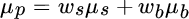
In Equation (2.1), equals the portfolio's expected return, equals the expected return of stocks, equals the expected return of bonds, equals the percentage of the portfolio allocated to stocks, and equals the percentage allocated to bonds.

As noted earlier, portfolio risk is a little trickier. It is defined as volatility, and it is measured by the standard deviation or variance (the standard deviation squared) around the portfolio's expected return. To compute a portfolio's variance, we must consider not only the variance of the asset class returns but also the extent to which they co‐vary. The variance of a portfolio of stocks and bonds is computed as follows:

(2.2)

Here equals portfolio variance, equals the standard deviation of stocks, equals the standard deviation of bonds, and equals the correlation between stocks and bonds.

Our objective is to minimize portfolio risk subject to two constraints. Our first constraint is that the weighted average of the stock and bond returns must equal the expected return for the portfolio. We are also faced with a second constraint. We must allocate our entire portfolio to some combination of stocks and bonds. Therefore, the fraction we allocate to stocks plus the fraction we allocate to bonds must equal 1.

We combine our objective and constraints to form the following objective function:

(2.3)

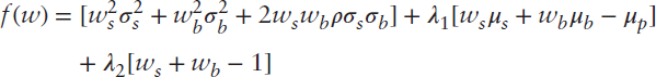
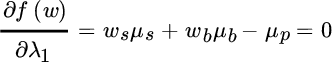
The first term of Equation (2.3) up to the third plus sign equals portfolio variance, the quantity to be minimized. The next two terms that are multiplied by represent the two constraints. The first constraint ensures that the weighted average of the stock and bond returns equals the portfolio's expected return. The Greek letter lambda () is called a Lagrange multiplier. It is a variable introduced to facilitate optimization when we face constraints, and it does not easily lend itself to economic interpretation. The second constraint guarantees that the portfolio is fully invested. Again, lambda serves to facilitate a solution.

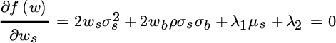
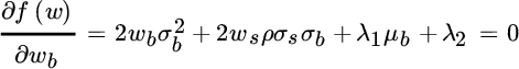
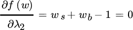
Our objective function has four unknown values: (1) the percentage of the portfolio to be allocated to stocks, (2) the percentage to be allocated to bonds, (3) the Lagrange multiplier for the first constraint, and (4) the Lagrange multiplier for the second constraint. To minimize portfolio risk given our constraints, we must take the partial derivative of the objective function with respect to each asset weight and with respect to each Lagrange multiplier and set it equal to zero, as shown below:

(2.4)

(2.5)

(2.6)

(2.7)

Given assumptions for expected return, standard deviation and correlation (which we specify later), we wish to find the values of and associated with different values of , the portfolio's expected return. The values for and are merely mathematical by products of the solution.

Next, we express Equations (2.4) (2.5), (2.6), and (2.7) in matrix notation, as shown below.

(2.8)

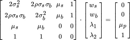
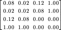
We next substitute estimates of expected return, standard deviation, and correlation for domestic equities and Treasury bonds shown earlier in Tables 2.1 and 2.2.

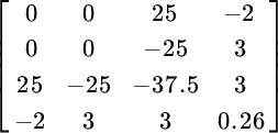
With these assumptions, we rewrite the coefficient matrix as follows:

Its inverse equals:

Because the constant vector includes a variable for the portfolio's expected return, we obtain a vector of formulas rather than values when we multiply the inverse matrix by the vector of constants, as shown below.

(2.9)

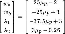
We are interested only in the first two formulas. The first formula yields the percentage to be invested in stocks in order to minimize risk when we substitute a value for the portfolio's expected return. The second formula yields the percentage to be invested in bonds. Table 2.3 shows the allocations to stocks and bonds that minimize risk for portfolio expected returns ranging from 9 to 12 percent.

TABLE 2.3 Optimal Allocation to Stocks and Bonds

Target Portfolio Return	9%	10%	11%	12%
Stock Allocation	25%	50%	75%	100%
Bond Allocation	75%	50%	25%	0%

The Sharpe Algorithm

In 1987, William Sharpe published an algorithm for portfolio optimization that has the dual virtues of accommodating many real‐world complexities while appealing to our intuition.⁸ We begin by defining an objective function that we wish to maximize.

(2.10)

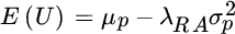
In Equation (2.8), equals expected utility, equals portfolio expected return, equals risk aversion, and equals portfolio variance.

Utility is a measure of well‐being or satisfaction, while risk aversion measures how many units of expected return we are willing to sacrifice in order to reduce risk (variance) by one unit. (Chapter 18 includes more detail about utility and risk aversion.) By maximizing this objective function, we maximize expected return minus a quantity representing our aversion to risk times risk (as measured by variance).

Again, assume we have a portfolio consisting of stocks and bonds. Substituting the equations for portfolio expected return and variance (Equations (2.1) and (2.2)), we rewrite the objective function as follows.

(2.11)

This objective function measures the expected utility or satisfaction we derive from a particular combination of expected return and risk, given our attitude toward risk. Its partial derivative with respect to each asset weight, shown in Equations (2.12) and (2.13), represents the marginal utility of each asset class.

(2.12)

(2.13)

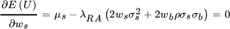
These marginal utilities measure how much we increase or decrease expected utility, starting from our current asset mix, by increasing our exposure to each asset class. A negative marginal utility indicates that we improve expected utility by reducing exposure to that asset class, while a positive marginal utility indicates that we should raise the exposure to that asset class in order to improve expected utility.

Let us retain our earlier assumptions about the expected returns and standard deviations of stocks and bonds and their correlation. Further, let's assume our portfolio is currently allocated 60 percent to stocks and 40 percent to bonds and that our aversion toward risk equals 2. Risk aversion of 2 means we are willing to reduce expected return by two units in order to lower variance by one unit.

If we substitute these values into Equations (2.12) and (2.13), we find that we improve our expected utility by 0.008 units if we increase our exposure to stocks by 1 percent, and that we improve our expected utility by 0.04 units if we increase our exposure to bonds by 1 percent. Both marginal utilities are positive. However, we can only allocate 100 percent of the portfolio. We should therefore increase our exposure to the asset class with the higher marginal utility by 1 percent and reduce by the same amount our exposure to the asset class with the lower marginal utility. In this way, we ensure that we are always 100 percent invested.

Having switched our allocations in line with the relative magnitudes of the marginal utilities, we recompute the marginal utilities given our new allocation of 59 percent stocks and 41 percent bonds. Again, bonds have a higher marginal utility than stocks; hence, we shift again from stocks to bonds. If we proceed in this fashion, we find when our portfolio is allocated to stocks and to bonds, the marginal utilities are exactly equal to each other. At this point, we cannot improve expected utility any further by changing the allocation between stocks and bonds. We have maximized our objective function.

By varying the values we assign to , we identify mixes of stocks and bonds for many levels of risk aversion, thus enabling us to construct the entire efficient frontier of stocks and bonds. Figure 2.1 shows the efficient frontier based on the expected returns, standard deviations, and correlations shown in Tables 2.1 and 2.2. All of the portfolios along the efficient frontier offer a higher level of expected return for the same level of risk than the portfolios residing below the efficient frontier.

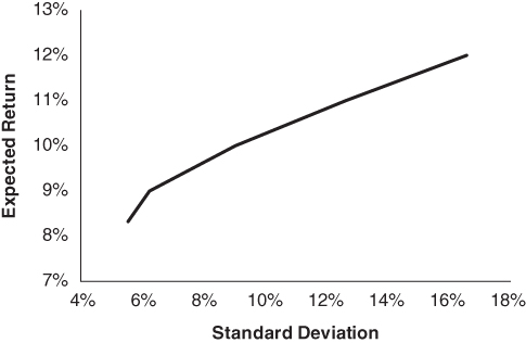
FIGURE 2.1 Efficient Frontier

Now let's consider the efficient frontier that is composed of the six asset classes specified in Tables 2.1 and 2.2. In particular, let's now focus on three efficient portfolios that lie along this efficient frontier: one for a conservative investor, one for an investor with moderate risk aversion, and one for an aggressive investor. Table 2.4 shows the three efficient portfolios.

TABLE 2.4 Conservative, Moderate, and Aggressive Efficient Portfolios

Asset Classes	Conservative	Moderate	Aggressive
U.S. Equities	15.9%	25.5%	36.8%
Foreign Developed Market Equities	14.5%	23.2%	34.5%
Emerging Market Equities	5.6%	9.1%	15.8%
Treasury Bonds	15.5%	14.3%	0.0%
U.S. Corporate Bonds	11.4%	22.0%	8.9%
Commodities	4.0%	5.9%	4.0%
Cash Equivalents	33.2%
Expected Return	6.0%	7.5%	9.0%
Standard Deviation	6.8%	10.8%	15.2%

The composition of these portfolios should not be surprising. The conservative portfolio has nearly a allocation to cash equivalents. The moderate portfolio is well diversified and not unlike many institutional portfolios. The aggressive portfolio, by contrast, has more than an 86 percent allocation to U.S. and foreign equities. It should be comforting to note that we did not impose any constraints in the optimization process to arrive at these portfolios. The process of employing an equilibrium perspective for estimating expected returns yields nicely behaved results.

The Optimal Portfolio

The final step is to select the portfolio that best suits our aversion to risk, which we call the optimal portfolio. As we discussed earlier in this chapter, the theoretical approach for identifying the optimal portfolio is to specify how many units of expected return we are willing to give up to reduce our portfolio's risk by one unit. We would then draw a line with a slope equal to our risk aversion and find the point of tangency of this line with the efficient frontier. The portfolio located at this point of tangency is theoretically optimal because its risk/return trade‐off matches our preference for balancing risk and return.

In practice, however, we do not know intuitively how many units of expected return we are willing to sacrifice in order to lower variance by one unit. Therefore, we need to translate combinations of expected return and risk into metrics that are more intuitive. Because continuous returns are approximately normally distributed,⁹ we can easily estimate the probability that a portfolio with a particular expected return and standard deviation will experience a specific loss over a particular horizon. Alternatively, we can estimate the largest loss a portfolio might experience given a particular level of confidence. We call this measure value at risk. We can also rely on the assumption that continuous returns are normally distributed to estimate the likelihood that a portfolio will grow to a particular value at some future date. Table 2.5 shows the likelihood of loss over a five‐year investment horizon for the three efficient portfolios, as well as value at risk measured at a 1 percent significance level, which means we are 99 percent confident that the portfolio value will not fall by more than this amount.

TABLE 2.5 Exposure to Loss

Risk statistics for end of five years
	Conservative	Moderate	Aggressive
Probability of Loss (return below 0%)	2.5%	6.7%	10.8%
1% Value at Risk	5.1%	17.0%	28.7%

If exposure to loss were our only consideration, we would choose the conservative portfolio, but by doing so we forgo upside opportunity. One way to assess the upside potential of these portfolios is to estimate the distribution of future wealth associated with investment in each of them.

Table 2.6 shows the probable terminal wealth as a multiple of initial wealth at varying confidence levels 15 years from now. For example, there is only a 5 percent chance that our nominal wealth would grow to less than 1.4 times initial wealth in 15 years, assuming we invest in the moderate portfolio. And there is a 5 percent chance (1 – 0.95) that our wealth could grow to a value as high as 5.2 times initial wealth.

TABLE 2.6 Distribution of Wealth 15 Years Forward (as a multiple of initial investment)

Terminal wealth, multiple, end of 15 years
Confidence Level	Conservative	Moderate	Aggressive
1%	1.3	1.1	0.9
5%	1.5	1.4	1.3
10%	1.7	1.7	1.6
25%	2.0	2.1	2.2
50%	2.3	2.7	3.2
75%	2.7	3.6	4.5
90%	3.2	4.5	6.3
95%	3.5	5.2	7.6
99%	4.1	6.8	11.0

These estimates of future wealth ignore any contributions or disbursements that may be added to or subtracted from the portfolios. To estimate future wealth taking cash flows into account, we would need to simulate the portfolios' performance between all cash flows throughout our investment horizon.

By mapping the portfolios' expected returns and standard deviations onto estimates of exposure to loss and the distribution of future wealth, we should have a clear idea of the merits and limitations of each portfolio. It is important to keep in mind, though, that there is no universally optimal portfolio; it is specific to each investor. If our focus is to avoid losses, the conservative portfolio might be optimal. If, instead, we believe that we can endure significant losses along the way in exchange for greater opportunity to grow wealth, then we might choose the aggressive portfolio. If our goal is to limit exposure to loss, yet still maintain a reasonable opportunity to grow wealth, then perhaps the moderate portfolio would suit us best.

Asset allocation is a complex process, yet one we should not ignore. Our intent in this chapter is to present the theoretical foundation of asset allocation as well as to discuss the practical implementation of this theory at its most basic level. In subsequent chapters, we describe various refinements to the basic approach described here. But before we move on to these refinements, we discuss some fallacies about asset allocation and do our best to dispel them.

REFERENCES

1. Levy, H., and H. Markowitz. 1979. “Approximating Expected Utility by a Function of Mean and Variance,” American Economic Review, Vol. 69, No. 3 (June).
2. Markowitz, H. 1952. “Portfolio Selection,” Journal of Finance, Vol. 7, No. 1 (March).
3. Sharpe, W. 1987. “An Algorithm for Portfolio Improvement,” Advances in Mathematical Programming and Financial Planning, Vol. 1 (Greenwich, CT: JAI Press Inc.).

NOTES

1. Markowitz (1952).

2. Levy and Markowitz (1979).

3. Kurtosis refers to the peakedness of a distribution. Kurtosis greater than three indicates that extreme returns are more likely than what one would expect from a normal distribution. Returns that are independent and identically distributed are likely to be normal.

4. This concept applies as well to any number of asset classes, but it is easier to visualize with only two asset classes.

5. See Chapter 1 for a detailed discussion of these characteristics.

6. Our empirical analysis is meant for illustration and we do not intend to offer conclusions about any specific portfolio, investment universe, or data set. We calibrate models and assumptions using reasonable market proxies such as the S&P 500 for U.S. equities; MSCI World ex US and MSCI emerging markets for foreign and emerging market equities; Bloomberg aggregate U.S. Treasury, corporate, and commodities benchmarks; and the risk‐free rate from Kenneth French's data website.

7. For those who care deeply about maximizing the portfolio's geometric mean, the arithmetic approach may still offer a reasonable approximation that can be tested for efficacy and compared to optimization with other, more complex numerical procedures.

8. See Sharpe (1987). Sharpe's algorithm can easily be adapted to accommodate transaction costs and allocation constraints.

9. A continuous return equals the natural logarithm of 1 plus the discrete return. It is the return, which, if compounded continuously, would give the discrete return. Continuous returns that are independent and identically distributed are normally distributed. It is therefore common practice to convert discrete returns, which are lognormally distributed owing to the effect of compounding, to continuous returns in order to estimate probabilities. We then convert the continuous return back to a discrete return by raising the base of the natural logarithm to the power of 1 plus the continuous return and subtracting 1.