CHAPTER 3
The Importance of Asset Allocation
FALLACY: ASSET ALLOCATION DETERMINES MORE THAN 90 PERCENT OF PERFORMANCE
No doubt, asset allocation is important, even critical, to investment success. Otherwise, why would we bother to write this book? Nonetheless, most investors, as well as academics, have a much inflated perception of the value of asset allocation compared to security selection.
THE DETERMINANTS OF PORTFOLIO PERFORMANCE
This misperception can be traced to an influential article published in the Financial Analysts Journal in 1986 called “The Determinants of Portfolio Performance.”1 The authors, Gary Brinson, Randolph Hood, and Gilbert Beebower, analyzed the performance of 91 large corporate pension plans during the 10‐year period from 1974 to 1983 in an effort to attribute their performance to three investment choices: asset allocation policy, timing, and security selection.
They defined the asset allocation policy return as the return of the long‐term asset mix invested in passive asset class benchmarks. They then measured the return associated with deviations from the policy mix assuming investment in passive benchmarks, and they attributed this component of return to timing. Finally, they measured the return associated with deviations from the passive benchmarks within each asset class and attributed this component of return to security selection. For each of the 91 funds, they regressed total return through time on these respective components of return. These regressions revealed that asset allocation policy, on average across the 91 funds, accounted for 93.6 percent of total return variation through time and in no case less than 75.5 percent.
Fundamental Flaw
This methodology is flawed because it presents no notion of a normal or a default asset mix. Their analysis implicitly assumes that the pension plans' funds would otherwise be uninvested, perhaps contained in a very large coffee can. Because the authors failed to net out an average or typical asset mix, most of the variation in performance that they attributed to asset allocation policy arose not from the choice of a portfolio's asset mix but, instead, from the decision merely to invest. The authors simply demonstrated that we incur risk when we invest in risky assets.
Imaginary World
To make our point as transparently as possible, consider the following hypothetical example. Imagine a world that has only two asset classes, stocks and bonds, with only two securities of equal size in each asset class.2 Figure 3.1 shows the performance of these two asset classes and of the securities within each asset class.

FIGURE 3.1 Regression of Portfolio Performance on Asset Class Performance
In this imaginary world, stocks and bonds as asset classes have the same performance each and every period. Moreover, Stock A has the same returns as Bond A, and Stock B has the same returns as Bond B. Whether you allocate 100 percent to stocks as an asset class or 100 percent to bonds as an asset class or to any combination in between, you will obtain the same performance each and every period and, on average, across all periods. In this imaginary world, asset allocation simply does not matter. It has no possible effect on performance. Security selection is the sole determinant of portfolio performance.
Now, imagine two investors. One investor is skillful; she chooses Stock A and Bond A. The other investor is unlucky; he chooses Stock B and Bond B.3 We need not specify the asset mixes chosen by these investors because all asset mixes yield the same performance. The performance of these two investors' portfolios is shown in Table 3.1.
TABLE 3.1 Imaginary Performance
| Period | Stock A | Stock B | Stock Index | Bond A | Bond B | Bond Index | Skillful Investor | Unlucky Investor |
| 1 | 15.0% | 7.5% | 11.3% | 15.0% | 7.5% | 11.3% | 15.0% | 7.5% |
| 2 | 8.0% | 4.0% | 6.0% | 8.0% | 4.0% | 6.0% | 8.0% | 4.0% |
| 3 | −1.0% | −0.5% | −0.8% | −1.0% | −0.5% | −0.8% | −1.0% | −0.5% |
| 4 | −14.0% | −7.0% | −10.5% | −14.0% | −7.0% | −10.5% | −14.0% | −7.0% |
| 5 | 4.0% | 2.0% | 3.0% | 4.0% | 2.0% | 3.0% | 4.0% | 2.0% |
| 6 | 32.0% | 16.0% | 24.0% | 32.0% | 16.0% | 24.0% | 32.0% | 16.0% |
| 7 | 18.0% | 9.0% | 13.5% | 18.0% | 9.0% | 13.5% | 18.0% | 9.0% |
| 8 | 6.0% | 3.0% | 4.5% | 6.0% | 3.0% | 4.5% | 6.0% | 3.0% |
| 9 | 24.0% | 12.0% | 18.0% | 24.0% | 12.0% | 18.0% | 24.0% | 12.0% |
| 10 | 8.0% | 4.0% | 6.0% | 8.0% | 4.0% | 6.0% | 8.0% | 4.0% |
| Average | 10.0% | 5.0% | 7.5% | 10.0% | 5.0% | 7.5% | 10.0% | 5.0% |
The difference in performance between the skillful investor and the unlucky investor is explained entirely by their respective choices of the individual securities. The fraction that they allocate to stocks as an asset class or to bonds as an asset class has no bearing whatsoever on their performance. Now let's apply the Brinson, Hood, and Beebower methodology to these portfolios to determine the extent to which their method would judge asset allocation to determine portfolio performance. They would calculate each investor's asset allocation return as the portfolio's asset weights applied to the stock and the bond asset class returns. They would then regress the investors' portfolio returns, shown in Table 3.1, on their asset allocation, which in this imaginary world is equivalent to regressing them on either the stock or the bond asset class returns, because all combinations of these asset class returns are the same in this imaginary world.
What would their methodology reveal? It would tell us that asset allocation determines 100 percent of the portfolios' performance and that none of the performance is determined by security selection. Figure 3.1 demonstrates this result, as it shows that all of the joint returns of portfolio performance and asset class performance lie precisely on the regression lines.
To prove our point as dramatically as possible, we contrived the security returns to be linearly related, thus showing the Brinson, Hood, and Beebower result to be in perfect opposition to the truth. We could also contrive a set of return series that had identical asset class returns but different security returns that were not linearly related. In this case, their methodology would show asset allocation to determine, say, 95 to 99 percent of performance when, in fact, it again would have no impact on performance.
The inescapable truth is that in an imaginary world in which asset allocation is unambiguously irrelevant and security selection is the sole determinant of portfolio performance, the methodology proposed by Brinson, Hood, and Beebower to attribute fund performance would show the exact opposite to be true.
THE BEHAVIORAL BIAS OF POSITIVE ECONOMICS
The Brinson, Hood, and Beebower methodology has another feature that limits its ability to separate the relative importance of various investment activities, which is also common to other methodologies that address this question. Most studies analyze the actual performance of funds.4 In this sense they are positive, as opposed to normative; they rely on actual returns that reflect some combination of the relative importance of alternative investment choices as well as the behavior of investors—that is, the extent to which investors choose to engage in various investment activities.
For example, some investors choose to invest in actively managed funds with high tracking error relative to the norm, but choose an asset mix that is close to the norm, such as the average asset mix of a relevant universe. Other investors choose actively managed funds with low tracking error relative to the norm, but choose an asset mix that is substantially different from the normal asset mix. In the former case, security selection will be seen to be more important than it is normally thought to be, while asset allocation will be seen to be less important than it is typically construed to be. In the latter case, the opposite will be true. But these conclusions could be misleading, because they may reflect as much or more about the investors' choices to emphasize asset allocation over security selection than the potential impact asset allocation and security selection actually have on portfolio performance.
To separate the intrinsic importance of an investment choice from an investor's decision to emphasize that choice, we need to measure the potential for an investment choice to cause dispersion in wealth. Dispersion is important to investors who believe they are skillful because it enables them to increase wealth beyond what they could expect to achieve by passive investment or from average performance. Dispersion is also important to investors who are unlucky because it exposes them to losses that might arise as a consequence of bad luck. As beneficial as it is for skillful investors to focus on activities that cause dispersion, it is equally important for unlucky investors to avoid activities that cause dispersion.
Determining Relative Importance Analytically
It is simple to measure the relative importance of asset allocation and security selection analytically if we limit our investment universe to two asset classes, each of which contains two securities. We simply measure the potential for dispersion as the tracking error between two investments that differ either by asset class composition or by security composition. We should expect security selection to cause greater dispersion than asset allocation because individual securities are more volatile than the asset classes that comprise them unless the securities move in perfect unison. Therefore, if we argue that asset allocation causes greater dispersion, we necessarily believe that high correlations among individual securities offset their relatively high individual volatilities.
Consider two asset classes that contain two securities each. Asset class A includes securities A1 and A2, while asset class B includes B1 and B2. We measure the relative volatility and, hence, the importance of security selection within asset class A as shown:
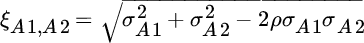
In Equation (3.1),  equals the relative volatility between
  and
and  ,
,  equals the standard deviation of
  ,
,  equals the standard deviation of
  , and
, and  is the correlation between
  and
and  . The same equation is used to calculate the relative volatility between securities B1 and B2.
We measure the importance of choosing between asset class A and asset class B the same way, but first we must calculate the standard deviation of each asset class. If we assume the individual securities are weighted equally within each asset class, the standard deviation of asset class A equals:

Here,  equals the standard deviation of asset class
  ,
,  equals the standard deviation of
  ,
,  equals the standard deviation of
  , and
, and  is the correlation between
  and
and  .
.
We repeat the same calculation to derive the standard deviation of asset class B.
The relative volatility between asset class A and asset class B equals:
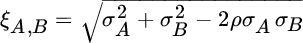
In Equation (3.3),  equals the relative volatility between A and B,
  equals the standard deviation of A,
  equals the standard deviation of B, and
  is the correlation between A and B.
Suppose the four securities are uncorrelated with each other. Then security selection would be more important than asset allocation because the asset classes would be less risky than the average risk of the securities they comprise, which results in less relative volatility between the asset classes than between the securities within each asset class. Moreover, as more securities are added, the asset class standard deviations decline further, which in turn further reduces the relative volatility between the asset classes. If, for example, security returns are uncorrelated and the securities are equally weighted, then the asset class standard deviation diminishes with the square root of the number of securities included. It is only when the correlation between asset classes A and B is substantially less than the correlation between the individual securities within the asset classes that the relative volatility between asset classes is greater than the relative volatility between securities. These relationships are illustrated in Table 3.2.
TABLE 3.2 Standard Deviation, Correlation, and Relative Volatility
| Standard Deviation | Correlation | Relative Volatility | Standard Deviation | Correlation | Relative Volatility | ||
| A1 | 10.0% | A1 | 10.0% | ||||
| A2 | 10.0% | 0.0% | 14.1% | A2 | 10.0% | 50.0% | 10.0% |
| B1 | 10.0% | B1 | 10.0% | ||||
| B2 | 10.0% | 0.0% | 14.1% | B2 | 10.0% | 50.0% | 10.0% |
| A | 7.1% | A | 8.7% | ||||
| B | 7.1% | 0.0% | 10.0% | B | 8.7% | 50.0% | 8.7% |
| Standard Deviation | Correlation | Relative Volatility | Standard Deviation | Correlation | Relative Volatility | ||
| A1 | 10.0% | A1 | 10.0% | ||||
| A2 | 10.0% | 50.0% | 10.0% | A2 | 10.0% | 50.0% | 10.0% |
| B1 | 10.0% | B1 | 10.0% | ||||
| B2 | 10.0% | 50.0% | 10.0% | B2 | 10.0% | 50.0% | 10.0% |
| A | 8.7% | A | 8.7% | ||||
| B | 8.7% | 33.3% | 10.0% | B | 8.7% | 25.0% | 10.6% |
The upper left panel shows that relative volatility between asset classes is less than relative volatility between securities when they are all uncorrelated with one another. The upper right panel shows the same result when they all are equally correlated with one another. The lower left panel shows the asset class and security correlations that lead to convergence between relative volatilities. Finally, the lower right panel provides an example in which the relative volatility between asset classes is higher than it is between securities.
Determining Relative Importance by Simulation
The associations between standard deviation, correlation, and relative volatility are easy to illustrate when we consider only two asset classes, each divided equally between only two securities. These associations become less clear when we consider several asset classes weighted differently among hundreds of securities with a wide range of volatilities and correlations. Under these real‐world conditions it is easier to resolve the question of relative importance by a simulation procedure known as bootstrapping.
Unlike Monte Carlo simulation, which draws random observations from a prespecified distribution, bootstrapping simulation draws random observations with replacement from empirical samples. Specifically, we generate thousands of random portfolios from a large universe of securities that vary only as a consequence of asset allocation or security selection. This allows us to observe the distribution of available returns associated with each investment decision as opposed to studying the actual performance of managed funds, which reflects the biases of their investors. Kritzman and Page (2002) conducted such an analysis for investment markets in five countries—Australia, Germany, Japan, the United Kingdom, and the United States—based on returns from 1988 to 2001. They showed that the dispersion around average performance arising from security selection was substantially greater than the dispersion arising from asset allocation in every country, and it was particularly large in the United States because the United States has a larger number of individual securities.5
L'Her and Plante (2006) refined the Kritzman and Page methodology to account for the relative capitalization of securities, and they also included a broader set of asset classes. Their analysis showed asset allocation and security selection to be approximately equally important—still a far different result than the conclusion of Brinson, Hood, and Beebower.
THE SAMUELSON DICTUM
We hope we have convinced you that asset allocation does not determine 94 percent of performance and that, contrary to this assumption, security selection has equal, if not greater, potential to affect the distribution of returns. Does it follow, therefore, that investors should focus more effort on security selection than asset allocation? Not at all. Paul A. Samuelson put forth the argument that investment markets are microefficient and macroinefficient, which implies that investors are more likely to succeed by engaging in asset allocation than in security selection. He argued that if an individual security is mispriced, a smart investor will notice and trade to exploit the mispricing, and by doing so will correct the mispricing. Therefore, opportunities to exploit the mispricing of individual securities are fleeting. However, if an aggregation of individual securities, such as an asset class, is mispriced, a smart investor will detect the mispricing and trade to exploit the mispricing. But one smart investor, or even several, would not have the scale to revalue an entire asset class. The mispricing of an asset class will likely persist until an exogenous shock jolts many investors, smart or not, to act in concert and thereby revalue the asset class. Thus, asset class mispricing endures sufficiently long to allow investors to profit from it.6
The bottom line is that asset allocation is very important, but not for the reasons put forth by Brinson, Hood, and Beebower.
REFERENCES
- G. P. Brinson and R. Hood. 2006. “Determinants of Portfolio Performance—20 Years Later: Authors' Responses,” Financial Analysts Journal, Vol. 62, No. 1 (January/February).
- G. P. Brinson, L. R. Hood, and G. L. Beebower. 1986. “Determinants of Portfolio Performance,” Financial Analysts Journal, Vol. 42, No. 4 (July/August).
- R. G. Ibbotson and P. D. Kaplan. 2000. “Does Asset Allocation Policy Explain 40, 90, or 100 Percent of Performance?” Financial Analysts Journal, Vol. 56, No. 1 (January/February).
- M. Kritzman. 2006. “Determinants of Portfolio Performance—20 Years Later: A Comment,” Financial Analysts Journal, Vol. 62, No. 1 (January/February).
- M. Kritzman and S. Page. 2002. “Asset Allocation versus Security Selection: Evidence from Global Markets,” Journal of Asset Management, Vol. 3, No. 3 (December).
- J. F. L'Her and J. F. Plante. 2006. “The Relative Importance of Asset Allocation and Security Selection,” Journal of Portfolio Management, Vol. 33, No. 1 (Fall).
- P. A. Samuelson. 1998. “Summing Up on Business Cycles: Opening Address,” in Beyond Shocks: What Causes Business Cycles, edited by J. C. Fuhrer and S. Schuh (Boston: Federal Reserve Bank of Boston).