Chapter 7
Option Strategies for Special Situations

Price action of risky assets in capital markets is anything but predictable with certainty. Companies announce changes in sales, profitability, products, policy, strategy, and capital structure all the time for example. Sometimes an investor doing his homework might be able to predict the probability of certain events occurring, but many if not most news events are a surprise catching the investor flatfooted. These corporate actions not only have an effect on the share price of the underlying stock, they have an effect on the price of options associated with those shares. Consequently, it is important to build intuition concerning option-pricing behavior in unusual circumstances. With this understanding, traders and investors will find opportunities from time to time that others will miss. Just as importantly, investors will avoid some of the pitfalls that cause unexpected but predictable losses with hindsight. The first situation discussed below concerns companies whose shares are heavily shorted. Stocks or other assets that are heavily shorted by speculators often behave differently than those that are not. In particular, they have the potential to become more volatile vis-à-vis historical experience and the distribution of potential returns can become skewed. Furthermore, it can cause the market to price options differently apart from a shift in implied volatility. With this knowledge, we can structure an option strategy to put the odds of success in the investor's favor to capitalize on this unique and temporary condition.

Second, we will also discuss skew more deeply. Skew changes the price and performance characteristics of certain options relative to their cohorts. These changes reveal shifts in investor sentiment concerning near-term price action of the underlying asset. The “signal” of stress or lack thereof expressed through the shape of the volatility surface often creates directional opportunity. To take advantage of that signal, we present a strategy designed to take advantage of this indicator of market stress.

Third, it is important to remember that the standard listed option in the United States allows for exercise at any time. While this does not affect the price behavior most of the time, it does so often enough to be an issue that must stay on our radar screen. One of the strategies institutional investors use to add value is called “dividend capture.” In theory, when a company pays a dividend, its price is supposed to fall by the amount of dividend paid. Academic studies show that stocks often fall less than the dividend paid. As a result, tax advantaged institutional investors like pension funds will buy a stock before the ex-dividend date, and flip the stock after the dividend is paid. (Tax laws require owners of stocks paying qualified dividends to hold the asset unhedged for at least 61 days out of a 121 day required holding period to enjoy favorable tax treatment of the dividend paid. So taxable entities usually do not participate in this activity.) For protection during this holding period, investors buy puts or sell calls to reduce or eliminate market risk from the strategy. With heavy demand for liquidity, price dislocations pop up from time to time, allowing speculators to get paid for providing liquidity to investors willing to pay for protection. Owners of calls do not have the right to the dividend paid by a company. To capture the dividend, the investor must exercise the option and settle the trade before the ex-dividend date. When a company pays a large special dividend, it might pay for the owners of an in- or at-the-money option to exercise their right early. Option sellers need to be aware of this phenomenon to avoid unexpected losses.

Option Strategy for Stocks under Heavy Short Interest

When companies falter (think Best Buy in 2011 and 2012) or are perceived to be way overpriced by some investors (think Tesla in the second half of 2013), they attract short sellers who want to take advantage of a potential fall in the price of a company's shares. Hedge funds do this by selling the company's shares short, which requires them to borrow stock. If too many hedge funds get the same idea, the amount of stock sold short becomes large relative to the total number of shares issued by the company. The measure of the quantity of shares that investors have sold short but not yet covered is known as the short interest. By itself, the number of shares sold short is not particularly meaningful, as the number of shares issued from one company to another differs. A more meaningful measure is known as the short interest ratio. It reveals the percentage of stock outstanding that is sold short. When the short interest ratio hits an extreme, there is the potential for a short squeeze. A short squeeze manifests as a sharp rise in the price of the asset sold short. It usually starts with a small rise in price. Short sellers, by their very nature, invest with a short time horizon. As they see price start to rise, they quickly get nervous and some will begin to cover their short position. As they do so, they push the price of a stock higher. Eventually, other short sellers panic and buy back their position at virtually any price. The end result it that the company's share price increases violently until the short sellers are squeezed out of their positions. Sometimes, other aggressive investors see the price spike and attempt to sell short at these higher prices. If the price continues to rise, these investors eventually exit their position at a loss before an even greater loss is suffered. At the extreme, this self-feeding loop can cause the price of an asset to rise far beyond a rational investor's view of value. This process continues until there are few if any short sellers or potential short sellers left.

Short squeezes represent a unique situation. Most investors do their homework and decide to buy an asset because they believe it is underpriced in the market place. They deliberately invest in the asset with the expectation that the price will rise to the value they place on the asset. Large institutional investors buy carefully, sometimes using trading algorithms to minimize their impact on price. When a short squeeze gets underway, short sellers buy for the exact opposite reason. They do not buy to take advantage of expected higher prices in the future; they buy to hide from higher prices. This makes the purchase an emotional one and the execution price is secondary to asset valuation.

Options provide a good way to play a potential short squeeze, as we can construct a strategy that has the potential for large gains with limited risk. One of the best strategies to capitalize on a potential price spike brought on by a short squeeze is to construct a short ratio call spread. To structure a short ratio call spread, sell an at-the-money call and buy two or more out-of-the-money calls. Don't be confused by the name. A short ratio call spread has both bullish and bearish implications. If the share price rises moderately, this spread will perform with bearish repercussions, as it will lose value. If the share price rises substantially, it will perform with bullish implications, and it has the potential to produce significant gains. There is always the possibility that a stock in a bearish trend will continue. The beauty of this strategy is that if it is properly structured, this strategy can allow for a nominal gain should the price of the stock stagnate or drift lower. As the options approach their expiration date, this allows the investor to reset strikes and expirations to new levels without suffering a loss due to time decay while awaiting the anticipated short squeeze and the outsized gains that come with it.

Consider company XYZ, whose stock exists with a heavy short interest that is currently trading for $25.00 a share. Exhibit 7.1 is an example of how we might want to structure a short ratio call spread to capitalize on a price spike resulting from a short squeeze. In this structure, we sell a three-month, at-the-money call, and buy two, three-month 12 percent out-of-the-money calls. Since a stock that is falling might continue to do so, we chose strikes and a ratio to enable the trade to profit if the stock price stagnates or trades down over the life of the spread.

	Sell	Buy	Net Credit
Number of Options	1	2
Strike	$25	$28
Risk-free Rate	2.00%	2.00%
Dividend	1.00%	1.00%
Time to Expiration	0.25	0.25
Volatility	35%	35%
Call Price	$1.77	$1.48	$0.29

Exhibit 7.1 Short 1 × 2 Ratio Call Spread, Stock Trading at $25 a Share

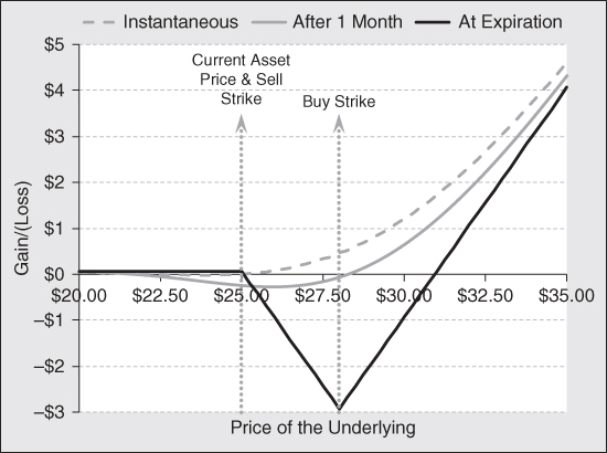
With this structure, the investor collects a $0.29 credit at the time the trade is initiated. This is the profit the investor will earn if the share price stagnates or falls, and the position is held to expiration. This is an important part of the structure as stocks that are heavily shorted are often in a downtrend, which usually continues until the selling stops. To attain this attribute, there is a trade-off between the ratio selected and the strike prices chosen, while still creating the opportunity for significant upside gains should a short squeeze manifest. The beauty of this structure is that it has a high probability of success. Probability theory tells us that there is a 66 percent chance the stock will be trading below $25.29 or above $30.71, which are the two breakeven points. Like any trade, this one is not guaranteed to be a winner, but the risk of loss is quite moderate if managed properly. Under the worst-case scenario, the price of the underlying increases to $28.00 a share at expiration. Under these circumstances, the trade loses $2.71. This return dynamic is revealed in the following chart showing the payoff pattern of this structure. But we should not hold the spread to expiration. The profit and loss dynamic indicates it should be rolled into new strikes and expirations each and every month.

The gray dotted line in Exhibit 7.2 shows the profit or loss we would experience given an instantaneous change in the price of the underlying security. Since the structure has positive delta, a gain will result if the price of the underlying asset rises. Furthermore, the structure has a very high gamma. This causes the delta to disappear quickly if the price of the underlying falls. If the price drop is significant, the delta of this structure turns negative and a gain occurs as well. The trade will suffer a very small nominal loss should the price of the underlying asset fall by a dollar or two.

Underlying	$20.00	$22.50	$25.00	$27.50	$30.00	$32.50	$35.00
% Change	−27%	−18%	−9%	0%	9%	18%	27%
Price	$0.10	$0.25	$0.29	−$0.06	−$1.02	−$2.55	−$4.52
Change (%)	−283	−517	−583	0	1583	4167	7450
Delta	−0.052	−0.057	0.045	0.257	0.505	0.713	0.851
Gamma	−0.014	0.015	0.066	0.098	0.095	0.069	0.042
Vega	−0.483	0.683	3.623	6.503	7.452	6.415	4.501
Theta	0.346	−0.470	−2.553	−4.622	−5.348	−4.671	−3.358

Exhibit 7.2 Profit/Loss on Short Ratio Call Spread

How this structure ages and how the price of the underlying moves is very important to the way it should be managed to minimize the potential for loss. Since the structure has positive gamma, the theta of this structure is negative (i.e., it will suffer time decay) when the trade is initiated, even though it starts out with a net credit. The process of decay turns to accretion after about a month or so, if the price of the underlying security does not change. To manage the trade, it is important to focus on the performance after a one-month holding period. The breakeven points over a one-month horizon are $23.00 and $27.75. Only a small loss occurs if the shares reside between these points over a one-month time horizon. Of note, the maximum loss we might suffer is just $0.24 a share. If the share price rises modestly, it is important to recognize that the time decay (theta) speeds up as the spread ages. Therefore, we should roll the spread by extending the expiration into new three-month options and adjust the strikes after a one-month holding period. If this is done, the investor eliminates the chance of a loss of any significance. If we let the position ride to expiration, we take the risk of suffering the maximum loss scenario. This analysis shows that there is no reason to take that chance. By holding the spread to expiration, we would lose if the share price trades above $25.00 a share and stays below $30.70 a share. Furthermore, we risk a substantial loss of $2.71 if the share price finds itself at $28 a share. Rolling avoids this potential.

The insight to this strategy is that it is a winner if the stock eventually has its big move. While waiting for this event, the investor is likely to suffer a string of small losses. To build some intuition around this phenomenon, it would be useful to walk through an example.

Exhibit 7.3 shows the results of a simulation of performing a monthly roll on this short 1 × 2 ratio call spread. In the first four months, the share price bounces around in a moderate trading range as the share price bleeds lower. Since these are small moves, time decay plays its part and a loss is suffered in these periods. In month 5, the share price reflects the short squeeze and a big gain is recorded. Over this five-month period, this strategy produced a total profit of $4.81. This is extraordinary, given the maximum expected monthly loss is just $0.24. The only scenario in which we suffer a loss is one where the short squeeze never takes place. While not a likely event, it certainly could happen. Given that one winner covers multiple small losers by many factors, a portfolio of these positions should be a winning strategy over time.

Beginning Values						Ending Values
Price	Sell Strike	Buy Strike	Sell 1	Buy 2	Net Credit	Price	Sell 1	Buy 2	Net Credit	Gain Loss	Cumulative Gain/Loss
25	25	28	1.77	0.74	0.29	27	2.72	1.13	0.46	−0.17	−0.17
27	27	30	1.91	0.85	0.21	26	1.08	0.34	0.40	−0.19	−0.36
26	26	29	1.84	0.80	0.24	25	1.02	0.30	0.42	−0.18	−0.54
25	25	28	1.77	0.74	0.29	24	0.97	0.27	0.43	−0.14	−0.68
24	24	27	1.70	0.68	0.34	35	11.05	8.10	−5.15	5.49	$4.81

Exhibit 7.3 Waiting for the Squeeze

To find stocks with short squeeze potential, investors should filter through a list of stocks with liquid listed options and identify the 10 to 20 companies with the highest short interest ratios and construct trades with structures similar to the one just presented. There is one caveat to keep in mind when employing this strategy: Do not overpay for volatility. The higher the iVol on the options traded, the lower the expected rate of return, as the investor needs a bigger move in price to capture a gain. Second, the item to keep an eye on is skew. In a “normal” situation, the iVol of the upside calls is lower than the at-the-money calls. If this is the case, the trade has a higher chance of succeeding than indicated above because the trader buys volatility at a lower price than he sells it. If, on the other hand, the skew takes the form of a volatility smile, this trade requires an investor to buy volatility more expensively than she sells it. This will work to dampen returns and reduce the probability of success. In short, this strategy works best when iVol is low and volatility skew has a normal shape for equities. This strategy will fight against significant headwinds when iVol is high and skew takes the form of a smile.

There are other filters we can use to improve the potential for success. For example, we might look at the valuation metrics of stocks with high short interest to identify the candidates that are more likely to enjoy a turnaround. When good news comes out on a company whose shares carry a high short interest ratio and whose shares trade with cheap valuation metrics, it is an elixir for explosive upward price movement.

Equities with high short interest are not the only situation for ratio spreads. This trade structure is applicable to other situations, such as when a biotech company is waiting for approval for a new drug that would substantially change the fortunes of the company. It is important to keep a creative mind when looking at unique situations to create option strategies that will maximize returns and minimize the risk of loss. Performance charts like the one in Exhibit 7.2 can be used to test strategies and manage time decay.

Opportunities in Skew

Option skew is best represented by the difference between the implied volatility for at-the-money put and call options and out-of-the-money puts or in-the-money calls. It is natural for options with moneyness of 80 or 90 percent to have a higher implied volatility than those with 100 percent moneyness. This is the market's way of expressing observed market dynamics in which prices tend to fall faster than they rise.

Most of the time, skew has little predictive power as an indicator for future price movements of an asset. However, when it hits a historical extreme, it can provide a strong clue that a change in trend might be at hand. When prices are in a downtrend, iVol tends to rise as investors look to put options to protect their existing positions. Some investors do not want to risk much premium, so they select out-of-the-money puts, which pushes up their price and skew. As a result, very high skew is associated with extremes in investor fear, and fear is associated with price bottoms. When markets are in an uptrend, investors are generally confident that prices will continue to rise. Consequently, they shy away from buying insurance. Option sellers participate in that confidence by freely offering put options for sale. They particularly like to sell downside puts as they expect stable or higher prices to cause those puts to expire worthless. This process drives down the absolute value of skew and lowers the volatility surface, as well. Thus, extraordinary low skew indicates complacency by market participants. When traders and investors become overconfident that a bull market will continue, they tend to act on feelings of greed, and buy without regard to price. This is the kind of market sentiment that is associated with a top in price.

Directional investors often seek out assets where volatility skew is at an extreme, as these are situations where the options market usually provides opportunity. Exhibit 7.4 is a chart of the price of gold overlaid on top of the corresponding historical skew for options on gold. Notice that skew was very low in August 2011 and this phenomenon occurred just at the time when the price of gold hit a peak. During the next nine months, skew fluctuated around its historical norm and the price of gold fluctuated randomly while falling during this period. In August 2012, skew once again collapsed during an uptrend in price. Depressed skew indicated a top was at hand. Predictably, the price of gold fell. This time prices fell in a relentless down trend that took the price of gold down 25 percent in a matter of just six months. In April 2013, skew moved to a record high, indicating investors were afraid the bear market would continue. Investors who follow skew would be on the lookout for a change in trend. The bottom was confirmed by a reduction in skew as prices began to move higher.

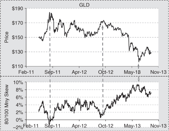
Exhibit 7.4 Price of Gold versus Skew

So how should an investor structure a trade when skew moves to an extreme high and they expect a change in price trend at any time? We know from the above analysis that skew will revert to the mean at some point. So we know iVol for options with moneyness less than 100 will fall more than options with moneyness of 100 or more. This tells us we definitely want to be a seller of options with moneyness less than 100 and a buyer of options with moneyness of 100 or higher. This way if the skew curve flattens, the price of the options sold will fall and the price of the options purchased will be relatively unaffected. Since the price of gold is depressed and skew is signaling a bottom could be at hand, we want the trade to profit from a rise in price. To do this, the resulting structure must be delta positive. iVol across the board is elevated and it is expected to fall as the price of gold rises. Therefore, we want the trade to be profitable as iVol falls and reverts to the mean as well. This tells us we are looking for a structure that is short vega. It often takes longer for a scenario to manifest than one expects. Option decay can kill the best-laid plans, so we need a structure that is either theta neutral and positive if possible. A potential trade structure that captures all these attributes is a call spread risk reversal. In this option structure, one buys an at-the-money call. To pay for that call, one simultaneously sells an out-of-the-money call (creating the call spread) and an out-of-the-money put (creating the risk reversal).

Exhibit 7.5 shows the valuation and performance metrics of this call spread risk reversal. This strategy meets all the criteria just outlined: positive delta, negative vega, and positive theta. The same amount of premium is collected on the options sold relative to the call purchased, resulting in no net debit or credit. Since April 2013 was a time of fear with respect to the gold market, downside puts traded with a significant skew. At-the-money options were priced with a 19 percent iVol, while 94.8 moneyness puts were priced at 22 percent. This volatility differential makes these puts relatively expensive allowing a seller to collect a relatively high premium. At the same time, skew drives down the iVol on upside call options, making them somewhat less expensive than at-the-money calls. At the end of the day, this structure allows the investor to buy options with 19 percent volatility and sell others with an average volatility of 20 percent.

	Buy	Sell	Sell	Net
Option Type	Call	Call	Put
Strike	$115	$121	109
Moneyness	100	105.2	94.8
Risk-free Rate	0.10%	0.10%
Dividend	0.00%	0.00%
Time to Expiration	0.25	0.25	0.25
Volatility	19.00%	18.00%	22%
Call Price	$4.37	$1.90	2.47	$0.00
Delta	0.52	0.30	–0.29	0.51
Vega	22.91	20.07	19.78	−16.94
Theta	−8.76	−7.26	−8.67	7.17

Exhibit 7.5 Call Spread Risk Reversal on GLD Trading at $115/Share

The selection of expiries depends on our expected price action, the level of implied volatility, and skew in the future. In this example, we selected a three month time to expiration, for consistency with the numerical examples presented throughout the book. However, one should look to longer expirations when the situation warrants. If we hold the opinion that volatility and skew will fall as the price of gold rises, we might want to use a longer-dated structure to gain from a drop in implied volatility. If we were to employ six-month options with the same strikes as above, the trade turns into one with a $1.62 credit. If the price of gold stays above $109 at expiration, the investor gets to keep that premium. If the iVol instantaneously falls by 200 basis points, skew falls from 9.5 percent to 4.75 percent, and the price of gold does not change, the net credit will fall to $0.78. This will allow the investor to exit the trade early and pocket the $0.84 per spread. Not only can the investor earn a return by a likely change in price, but by skew and iVol returning to normal levels as well.

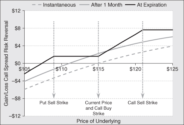
Exhibit 7.6 shows the total return profile of this longer six-month call spread risk reversal. This structure has positive theta initially so it will tend to rise in value over time. If the price of gold rises, the positive delta of 0.49 ensures this structure will be a winner immediately. Since the investor is writing an upside call, the maximum amount one can earn is $7.62 (call upper strike-call lower strike-premium) per spread. As long as the price of GLD does not fall below $107.38, which is the strike of the downside put less the premium collected, the trade will generate a gain. Below that point, the investor will suffer a loss. In the final analysis, the risk/reward of this trade is attractive. So long as the price of GLD does not fall more than 6.63 percent at expiration, the investor will be rewarded for the risk taken. A drop in iVol and/or skew before expiration provides another way the investor can profit from this structure.

Underlying	$100.00	$105.00	$110.00	$115.00	$120.00	$125.00	$130.00
% Change	−13%	−9%	−4%	0%	4%	9%	13%
Price	−$11.20	−$7.55	−$4.34	−$1.62	$0.59	$2.31	$3.58
Change (%)	591	366	168	0	−137	−243	−321
Delta	0.772	0.688	0.594	0.494	0.392	0.297	0.214
Gamma	−0.016	−0.018	−0.020	−0.020	−0.020	−0.018	−0.015
Vega	−17.737	−21.724	−25.334	−27.976	−28.964	−27.917	−24.997
Theta	3.937	4.754	5.420	5.839	5.914	5.601	4.952

Exhibit 7.6 Profit/Loss Six-Month Call Spread Risk Reversal on GLD

There are other strategies investors can use, of course. One could simply sell a six-month, $109 strike put and hope the price is above this level at expiration. In this case, the investor would keep the $4.33 premium collected. The breakeven point of this trade is $104.67, which is 9.0 percent less than the going price of GLD. Investors who are more risk averse might select a lower strike. Naturally, they would have to accept a lower premium. Those who are more risk tolerant might choose a higher strike and collect a higher premium.

Exhibit 7.4 shows that there are times of extremely low skew, as well. August 2011 and July 2012 is a perfect examples of a time when skew went far below its historical norm—in fact, it briefly went negative in 2011. This represents another special situation that option investors can capitalize on. So how should an investor structure a trade in gold options when skew is severely depressed? Skew is a mean reverting variable so, the investor should expect it to increase over time. As a result, iVol for options with moneyness less than 100 will rise more than options with moneyness of 100 or more. This tells us we definitely want to be a buyer of options with moneyness less than 100 and a seller of options with moneyness of 100 or higher. This way, if the skew curve steepens, the price of the options purchased will rise and the price of the options sold will stay the same or fall. Since the price of gold is elevated after a sharp bull move and skew is signaling a change in trend, we want the trade to profit from a fall in price. To do this, the resulting structure must rise when the price of GLD falls (i.e., possess a negative delta). iVol across the board is depressed and it is expected to rise as the price of gold falls. Therefore, we want the trade to be profitable as iVol increases and reverts to the mean as well. This tells us we are looking for a structure that is long vega. We want to avoid time decay, and profit from it if possible, so we need a structure that is either theta neutral or, better yet, positive. A trade structure that captures all these attributes is a short ratio put spread. In this option structure, the investor sells an at-the-money put and uses some or all of the proceeds to purchase downside puts.

Exhibit 7.7 shows the valuation and performance metrics of this 1 × 3 short ratio put spread. This strategy meets the primary criteria outlined, namely, negative delta and positive vega. Theta is problematic, at least initially, as it starts out negative. Far more premium is collected than spent, resulting is a credit of $1.79. This will cause theta to eventually become positive, as the spread ages under the scenario where the price of gold stagnates or continues to rise. Be aware, however, that it becomes increasingly negative should the price of gold fall. Since September 2012 was a time of euphoria with respect to the gold market, downside puts trade at a significant discount. At-the-money options were priced with an 18.0 percent iVol, while 91.8 percent moneyness puts were priced at just 18.5 percent. At the end of the day, this structure allows the investor to buy volatility cheap and sell it expensively on a historical basis. As a final thought, extending the time to expiration from three months to six months turns this trade from a net credit of $1.79 to a net debit of $1.17, making it more costly to put on. This structure has a bigger negative delta and more vega, which is good, but it comes with more time decay. At the end of the day, how one structures a trade is a personal choice. While it may not appear that the investor are compensated for the additional time decay by extending time to expiration. However, the loss in a worst case scenario is less, so there is an offsetting benefit.

	Sell	Buy	Net
Option Type	Put	Put
Number of Options	1	3
Strike	$170	$156
Moneyness	100	91.8
Risk-free Rate	0.10%	0.10%
Dividend	0.00%	0.00%
Time to Expiration	0.25	0.25
Volatility	18.00%	18.50%
Call Price	$6.08	$1.43	–$1.79
Delta	−0.48	−0.16	−0.00
Gamma	0.03	0.02	0.03
Vega	33.87	21.02	29.19
Theta	−12.11	−7.75	−1.51

Exhibit 7.7 Short 1 × 3 Ratio Put Spread with Gold at $170/Ounce

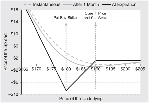
Exhibit 7.8 shows the total return profile of the three-month short 1 x 3 ratio put spread. This structure has negative theta initially so it will tend to fall in value over the initial phase of the trade. Since the structure pays a net credit, theta eventually become positive and introduces a slight boost to returns. If the price of gold falls, the negative delta and positive gamma make this trade a winner immediately. The beauty of this structure is that the investor still earns a profit if they are too early, which happens quite often in manias. If held to expiration, the investor will keep the premium collected in a bullish scenario. Nonetheless, investors should probably roll the structure to new strikes and expirations after a month should the price of gold rise. Remember, if investors are expecting a sharp drop in price, they should have an optimal structure to capitalize on it.

Underlying	$155.	$160.	$165.	$170.	$175.	$180.	$185.
% Change	−9%	−6%	−3%	0%	3%	6%	9%
Price	$2.57	−$0.09	−$1.43	−$1.79	−$1.65	−$1.29	−$0.88
Change (%)	−244	−95	−20	0	−8	−28	−51
Delta	−0.689	−0.386	−0.157	−0.011	0.061	0.082	0.074
Gamma	0.066	0.054	0.037	0.021	0.008	0.001	−0.003
Vega	73.580	64.650	48.046	29.185	12.886	1.704	−4.187
Theta	−27.307	−24.121	−18.069	−11.137	−5.106	−0.931	1.308

Exhibit 7.8 Profit/Loss Short Three-Month 1 × 3 Ratio Put Spread on GLD

There are other strategies investors can use, of course. One alternative is to simply sell a 180-strike call and hope the price of gold stays below this level at expiration. In this case, we would keep the $2.52 premium. The breakeven point of this trade is $182.52, which is 6.9 percent higher than the going price of GLD. Those who are more risk averse might select a higher strike. Naturally, they would have to accept a lower premium. Those who are more risk tolerant might choose a lower strike and collect a higher premium. This is a very dangerous trade, however, as huge price moves can accompany a mania before it ends. This is the lesson learned from the dotcom bubble of 1997 to 1999 and the real estate bubbles for 2000 to 2007. We recommend investors stay with risk-limiting structures like the one suggested above.

Dividend Capture

Investors who purchase common stock are entitled to the dividend, if any, paid by the company. Investors in call options, on the other hand, are not entitled to the dividend because they do not own the stock yet. If the owner of a call wants the dividend, they must exercise their option and take ownership of the shares before the ex-dividend date. This being the case, the market prices of puts and calls reflect the market's expectation of the stream of dividends the company pays over the life of the options. Taking into account discreet dividends is a bit tricky, as the investor must have a sound estimate of the dividend to be paid and the date on which it will be paid.

The B–S–M model is a method of pricing a European option, which cannot be exercised early. Listed options on stocks of individual companies that trade in the United States are American-style options, which are exercisable at any time before the option expires. Most of the time, the B–S–M will price American options correctly, as an option always has time value. Therefore, it is usually better to sell an option than to exercise it early. This condition can break down the day before the ex-dividend date. If the dividend is large enough, such as when a special dividend paid as part of a corporate financial restructuring, it might be optimal to exercise in-, at-, or near-at-the-money options before their expiration date.

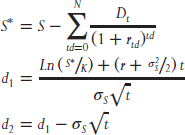
Setting aside the issue of early exercise for a moment, we can modify the B–S–M option-pricing model to take into account discrete dividends payable on specific dates. The most common technique practitioners' use is called the dividend escrow method. This method assumes that the dividends are known in advance and when they will be paid with certainty. Using this approach, we simply replace the current price of the stock S, with S minus the present value of the dividend stream expected over the life of the option. Now that the dividends have been accounted for in a discrete fashion, the dividend yield is no longer part of the mathematical relationship. By making these substitutions, the following are the formulas we should use when pricing options that pay discreet dividends.

Black–Scholes–Merton Option-Pricing Model for a Company or Index Paying Discrete Dividends

1. 

with the boundary condition that at expiration.

with the boundary condition that 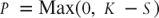at expiration.

where:

C	=	Price of a call option
P	=	Price of a put option
S	=	Current price of the stock or index
K	=	Strike price of the option
Dtd	=	Dividend paid at time td
r	=	Risk-free rate
t	=	Time to option expiration
td	=	Time to dividend payment
	=	Standard deviation of asset returns
N( )	=	Cumulative standard normal distribution function

To price the option correctly using the escrowed dividend model, we must value the option in two distinct ways. We must value the option on the day before the stock goes ex-dividend and repeat the process by valuing the option to its expiration date. The true value of the option is the higher of these two figures. Take the following example where a three-month option goes ex-dividend the day before option expiration.

The analysis in Exhibit 7.9 shows that the B–S–M option model incorporating discrete dividends would price the call at $3.44. If the option could not be exercised early, this would be a fair price as the owner of the option could not exercise their right and collect the dividend. If the option is priced as if it expires the day before the dividend is paid, its value is $5.12. It is higher, because the owner of the option could exercise and capture the dividend if it made sense to do so. Therefore, the fair value of an American option is equal to $5.12, as it can be sold or exercised anytime before the dividend is paid. Said another way, the difference between the value of an American and European option is $1.68.

	Value to Expiration	Value Day Before Ex-Dividend Date
Stock Price	$100
Strike Price	$102
Interest Rate	1%
Volatility	30%
Time to Dividend	89 days
Time to Expiration	90 days	89 days
Dividend	$4.00	0.00
Value of a Call	$3.44	$5.12

Exhibit 7.9 Valuing a Call Option with Discreet Dividends

When applying the escrow method, we are implicitly making the assumption that the dividend payments are known in advance with certainty. As we all know, companies change their dividend payments all the time. When companies are doing well and management believes that their prosperity will continue, they will increase their dividend. We know from option-pricing theory that for a given share price, an increase in the dividend will reduce the value of a call option and increase the value of a put option because the price of the stock falls by the dividend amount when the stock goes ex-dividend. But a permanent increase in the dividend is a signal to investors that management expects good times to continue and for earnings to grow. This entices investors to push up the price of the stock, which drives up the price of a call and pushes down the price of a put. This is generally not the case when the company pays a special one-time dividend.

Special one-time dividends are rare, but there are unique situations where a company might choose to do so. One reason for a special dividend occurs when market actors believe there will be a change in the tax law applied to dividend payments. In 2012, for example, dividend payments were taxed at the long-term capital gains tax rate and not the personal tax rate on ordinary income. This means that when a company paid a dividend, investors would have to pay an income tax of no more than 15 percent of the dividend amount, which was far less that the rate on ordinary income of 39.6 percent. The law that established the preferential tax treatment of dividends was set to expire at the end of the year. When it did, dividends for 2013 and beyond would be taxed at the marginal tax rate for ordinary income, which could be as high as 39.6 percent. Since dividends paid to shareholders are not tax deductible at the corporate level, they do not reduce a company's income tax liability. As a result, shareholders were better off getting paid dividends sooner rather than later. At the same time, many large capitalization companies were holding a great deal of cash on their balance sheet. Others had little or no debt on their books. As a result, many companies had the ability to pay dividends out of cash on the balance sheet. Super low interest rates allowed companies without excess cash to borrow and payout the proceeds.

When these companies announced a special dividend to be paid before year-end, it did not have a permanent effect on the company's stock, as it did not represent a signal about rosier future prospects of the company. It could, however, have a material effect on the value of listed options. Take the situation where an investor holds a 90-day option on a company that usually pays a $1.00 per share dividend, and the company announces that it will accelerate $2.00 per share of future dividends into the current dividend payment of $1.00 scheduled for payment in 30 days.

Exhibit 7.10 shows that if investors were holding a European at-the-money call option on the day the accelerated dividend was announced, they would have suffered an immediate loss of $0.96 (5.53 − 4.57). This analysis points out the importance of monitoring the political landscape for potential changes in tax laws that can temporarily change a company's dividend policy. Buyers of calls also need to pay close attention to management's propensity to give excess cash back to shareholders on a one-time basis as part of a financial restructuring as well. If we anticipated this change, the optimal strategy would be to sell calls and buy stock on a delta-neutral basis. With this strategy, the investor would be hedged against random movements in the price of the underlying stock while capturing a potential windfall from a sharp drop in premium. The effect on the price of a put is equally dramatic. By lowering the forward price of the underlying instrument, the value of an at-the-money put would increase by $1.04 (7.32-6.28). In the end, a special dividend could result in a wealth transfer from call buyers to put buyers, and from put sellers to call sellers. The loss above could be avoided if the owner held an American-style option and they exercised early. So options traders must be aware of when it is appropriate to exercise early.

	Value to Expiration	Value Day Before Ex-Dividend Date
Stock Price	$100
Strike Price	$100
Interest Rate	1%
Volatility	30%
Time to Dividend	30 days
Time to Expiration	90 Days
Dividend	$1.00	$3.00
Value of a Call	$5.53	$4.56
Value of a Put	$6.28	7.32

Exhibit 7.10 Change in Valuation of a Call Option Incorporating a Special Dividend

While the math of special dividends is straightforward, the regulations around that special dividend are more complicated. As a result of this episode with accelerated dividends, regulators in the United States have changed the rules concerning accelerated dividends. Currently in the United States, if the amount of the special dividend is more than $12.50 per contract ($0.125 per share for most option contracts), the strike price will be reduced by the amount of the special dividend. This eliminates the effect of the special dividend on the price of an option. It is important to remember that the rules concerning special dividends differ by country and they change over time. To stay abreast of these rules, investors should visit the website of the local regulatory bodies. For U.S. investors, that would be the OCC.

Listed options that trade on U.S. exchanges are American-style options that give the owner the opportunity to exercise anytime before or at expiration. It is rarely if ever optimal to exercise an option early on a stock that does not pay a dividend. For options on stocks that do pay a dividend, there are circumstances when the investors should exercise early to capture the dividend and avoid losing money. As already shown, cash dividends affect the price of an option because the price of the stock is expected to fall by the dividend amount on the ex-dividend date.

The question is, “When should we exercise an option early?” In option speak, we should exercise an option early when the theoretical value of the option is at parity (i.e., there is no time value) and the option's delta is 1.0. While this might not be particularly helpful for the novice, an example should add clarity. For simplicity in Exhibit 7.11, we will look at an deep in the money call option with two days to expiration and one day to the ex-dividend date.

	Value to Expiration	Value Day Before Ex-Dividend Date
Stock Price	$100
Strike Price	$90
Interest Rate	1%
Volatility	30%
Time to Dividend	1 days
Time to Expiration	2 days
Dividend	$2.00	$0.00
Value of a Call	$8.00	$10.00
Delta	1.00	1.00

Exhibit 7.11 Valuing of a Call Option the Day before a Special Dividend

The value of this call option the day before the ex-dividend date is $10.00. This must be the case because we could buy the call for $10.00, immediately exercise the option at $90.00, sell the stock immediately for $100.00, and be left with $0.00. If the option had a lower price, an arbitrage opportunity would exist. Even though the option is fairly priced at $10.00 and an arbitrage opportunity does not exist, this is a situation where an existing owner of the call would find it in their best interest to exercise the option anyway.

If the owner of the call does nothing, the stock would fall by $2.00 on the ex-dividend date and so would the price of the option. In this case, the owner of the call would lose $2.00 overnight. If the owner of the call exercises early, they now own the stock at a cost of $100.00, and could sell it for the same price. When the stock goes ex-dividend the next day, it will trade for $98.00, resulting in a $2.00 capital loss. This loss, however, is offset by the $2.00 dividend and the owner retains a total value of $100.00. The investor is not better off because he makes a profit, he is better off because he avoids a loss. If, for some reason, the option were trading at $9.50, which is below parity, the investor should immediately buy the call and exercise it. Under this scenario, we would pocket $0.50 (100 − 90 − 9.50). Bear in mind that options rarely trade at or below parity because the arbitrageurs and market makers step in and push the price of the option to at least parity. If the option were trading slightly above parity at $10.50, the investor would lose $0.50 (100 − 90 − 10.50) if they did exercised early. This, however, is a better choice than holding the option and suffering a $2.50 loss.

This might seem like an interesting theoretical artifact of the option market, but this has real-life implications. Market makers and institutional investors often write call options on stocks that pay big dividends hoping some fraction of the option buyers do not exercise their right before the ex-dividend date. When this happens, this results in a windfall profit for the option seller. Many option buyers who forgot to exercise their options before the ex-dividend dates in late 2012 suffered a heavy price.

Final Thought

Active investors find that interesting situations come up all the time. If they have a good idea of how a situation will play out, they can combine options in many different ways to take advantage of their insight. We think it is very important to look at scenario analysis like those shown in the charts above to see the potential gains and losses given various structures. This way, they can make an educated judgment concerning risk and return. Options are complicated instruments and one must be cognizant of the intricacies concerning their mechanics particularly as it concerns dividends. As a result, investors must be deeply aware of actions management might take concerning one-off events like takeovers and capital restructurings. With a proper understanding of these issues, the investor will reduce the chances of getting blindsided and if they are nimble enough, profit from special situations.