Looking Inside
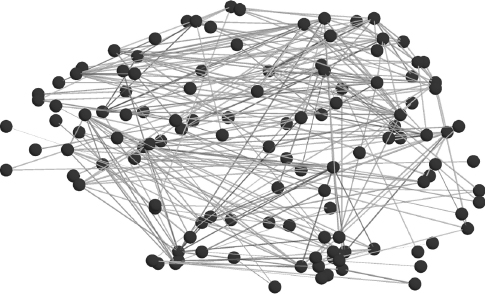
The above-mentioned projects, and many other projects that address similar matters, use various technologies to derive detailed information about the brains of humans, primates, and other model organisms. Common to many of these projects are the techniques used to obtain information about brain structures and even, in some cases, about neuron-level connectivity.
In this section we will consider imaging methods that can be used, in non-invasive ways, to obtain information about working brains in order to observe their behavior. Such methods are known as neuroimaging. When the objective is to obtain detailed information about the three-dimensional structure and composition of brain tissues, it is useful to view the brain as divided into a large number of voxels. A voxel is the three-dimensional equivalent of a pixel in a two-dimensional image. More precisely, a voxel is a three-dimensional rectangular cuboid that corresponds to the fundamental element of a volume, with the cuboid dimensions imposed by the imaging technology. Cuboid edge sizes range from just a few nanometers to a centimeter or more, depending on the technology and the application. Smaller voxels contain fewer neurons on average, and correspond to lower levels of neuronal activity. Therefore, the smaller the voxels, the harder it is to obtain accurate information about their characteristics using imaging techniques that look at the levels of electrical or chemical activity. Smaller voxels also take longer to scan, since scanning time, in many technologies, increases with the number of voxels. With existing technologies, a voxel used in the imaging of live brains will typically contain a few million neurons and a few billion synapses, the actual number depending on the voxel size and the region of the brain being imaged. Voxels are usually arranged in planes, or slices, which are juxtaposed to obtain complete three-dimensional information about the brain. Many of the techniques used to image the brain are also used to image other parts of the body, although some are specifically tuned to the particular characteristics of brain tissue.
Neuroimaging uses many different physical principles to obtain detailed information about the structure and behavior of the brain. Neuroimaging can be broken into two large classes: structural imaging (which obtains information about the structure of the brain, including information about diseases that manifest themselves by altering the structure) and functional imaging (which obtains information about brain function, including information that can be used to diagnose diseases affecting function, perhaps without affecting large structures).
Among the technologies that have been used in neuroimaging (Crosson et al. 2010) are computed tomography (CT), near-infrared spectroscopy (NIRS), positron-emission tomography (PET), a number of variants of magnetic-resonance imaging (MRI), electroencephalography (EEG), magnetoencephalography (MEG), and event-related optical signal (EROS).
Computed tomography (Hounsfield 1973), first used by Godfrey Hounsfield in 1971 at Atkinson Morley’s Hospital in London, is an imaging technique that uses computer-processed x-ray images to produce tomographic images which are virtual slices of tissues that, stacked on top of each other, compose a three-dimensional image. X rays with frequencies between 30 petahertz (3 × 10¹⁶ Hz) and 30 exahertz (3 × 10¹⁹ Hz) are widely used to image the insides of objects, since they penetrate deeply in animal tissues but are attenuated to different degrees by different materials.
Tomographic images enable researchers to see inside the brain (and other tissues) without cutting. Computer algorithms process the received x-ray images and generate a three-dimensional image of the inside of the organ from a series of two-dimensional images obtained by sensors placed outside the body. Usually the images are taken around a single axis of rotation; hence the term computed axial tomography (CAT). Computed tomography data can be manipulated by a computer in order to highlight the different degrees of attenuation of an x-ray beam caused by various body tissues. CT scans may be done with or without the use of a contrast agent (a substance that, when injected into the organism, causes a particular organ or tissue to be seen more clearly with x rays). The use of contrast dye in CT angiography gives good visualization of the vascular structures in the blood vessels in the brain.
Whereas x-ray radiographs have resolutions comparable to those of standard photographs, computed tomography only reaches a spatial resolution on the order of a fraction of a millimeter (Hsieh 2009). A CT scan takes only a few seconds but exposes the subject to potentially damaging ionizing radiation. Therefore, CT scans are not commonly used to study brain behavior, although they have provided important information about brain macro-structures. CT scans are used mostly to determine changes in brain structures that occur independently of the level of activity.
Because the characteristics of the tissue change slightly when the neurons are firing, it is possible to visualize brain activity using imaging techniques. One of the most significant effects is the change in blood flow. When a specific area of the brain is activated, the blood volume in the area changes quickly. A number of imaging techniques, including NIRS, PET, and MRI, use changes in blood volume to detect brain activity. The fact that water, oxygenated hemoglobin, and deoxygenated hemoglobin absorb visible and near-infrared light can also be used to obtain information about the location of neuronal activity.
Blood oxygenation varies with levels of neural activity because taking neurons back to their original polarized state after they have become active and fired requires pumping ions back and forth across the neuronal cell membranes, which consumes chemical energy. The energy required to activate the ion pumps is produced mainly from glucose carried by the blood. More blood flow is necessary to transport more glucose, also bringing in more oxygen in the form of oxygenated hemoglobin molecules in red blood cells. The blood-flow increase happens within 2–3 millimeters of the active neurons. Usually the amount of oxygen brought in exceeds the amount of oxygen consumed in burning glucose, which causes a net decrease in deoxygenated hemoglobin in that area of a brain. Although one might expect blood oxygenation to decrease with activation, the dynamics are a bit more complex than that. There is indeed a momentary decrease in blood oxygenation immediately after neural activity increases, but it is followed by a period during which the blood flow increases, overcompensating for the increased demand, and blood oxygenation actually increases after neuronal activation. That phenomenon, first reported by Seiji Ogawa, is known as the blood-oxygenation-level-dependent (BOLD) effect. It changes the properties of the blood near the firing neurons. Because it provides information about the level of blood flow in different regions of the brain, it can be used to detect and monitor brain activity (Ogawa et al. 1990). The magnitude of the BOLD signal peaks after a few seconds and then falls back to a base level. There is evidence that the BOLD signal is more closely related to the input than to the output activity of the neurons in the region (Raichle and Mintun 2006). In parts of the cortex where the axons are short and their ends are near the neuron bodies, it makes no difference whether the BOLD signal is correlated with the input or with the output of the neurons, since the voxels are not small enough to distinguish between the different parts of the neuron. In other areas of the brain, where the axons are longer, the difference between input and output activity can be significant.
Obtaining accurate measures of the level of the BOLD signal is difficult, since the signal is weak and can be corrupted by noise from many sources. In practice, sophisticated statistical procedures are required to recover the underlying signal. The resulting information about brain activation can be viewed graphically by color coding the levels of activity in the whole brain or in the specific region being studied. By monitoring the BOLD signal, it is possible to localize activity to within millimeters with a time resolution of a few seconds. Alternative technologies that can improve both spatial resolution and time resolution through the use of biomarkers other than the BOLD signal are under development, but they have other limitations. Therefore, the majority of techniques used today use the BOLD signal as a proxy for brain activity.
Near-infrared spectroscopy (NIRS) is a technique based on the use of standard electromagnetic radiation that uses a different part of the spectrum than CT techniques use: the range from 100 to 400 terahertz (that is, from 1 × 10¹⁴ to 4 × 10¹⁴ Hz). NIRS can be used to study the brain because transmission and absorption of NIR photons by body tissues reveal information about changes in hemoglobin concentration (Villringer et al. 1993). NIRS can be used non-invasively to monitor brain function by measuring the BOLD signal because in the NIRS frequency range light may diffuse several centimeters through the tissue before it is diffused and detected (Boas, Dale, and Franceschini 2004). A NIRS measurement consists in sending photons of appropriate frequency into the human brain, sensing the diffused light, and using computer algorithms to compute the densities of substances causing the photons to diffuse.
NIRS is sensitive to the volume of tissue residing between the source of light entering the tissue and the detector receiving the light that diffuses out of the tissue. Since NIR light penetrates only a few centimeters into the human brain before being diffused, the source and the detector are typically placed on the scalp, separated by a few centimeters. The resulting signal can be used to image mainly the most superficial cortex. NIRS is a non-invasive technique that can be used to measure hemodynamic signals with a temporal resolution of 100 Hz or better, although it is always limited by the slow response of the BOLD effect. Functional NIR imaging (fNIR) has several advantages in cost and portability over MRI and other techniques, but it can’t be used to measure cortical activity more than a few centimeters deep in the skull, and it has poorer spatial resolution. The use of NIRS in functional mapping of the human cortex is also called diffuse optical tomography (DOT).
Positron-emission tomography (PET) is a computerized imaging technique that uses the particles emitted by unstable isotopes that have been injected into the blood. The technique is based on work done by David Kuhl, Luke Chapman, and Roy Edwards in the 1950s at the University of Pennsylvania. In 1953, Gordon Brownell, Charles Burnham, and their group at Massachusetts General Hospital demonstrated the first use of the technology for medical imaging (Brownell and Sweet 1953).
PET is based on the detection of pairs of high-energy photons emitted in the decay of a positron emitted by a radioactive nucleus that has been injected into the body as part of a biologically active molecule. A positron is a sub-atomic particle with the same mass as an electron, but with positive charge. It is, in fact, a piece of antimatter—an anti-electron. When emitted from a decaying radionuclide integrated in ordinary matter, a positron can travel only a very short distance before encountering an electron, an event that annihilates both particles and results in two high-energy photons (511 KeV, or kilo-electron-volts) leaving the site of annihilation and traveling in opposite directions, almost exactly 180 degrees from one another. Three-dimensional images of the concentration of the original radionuclide (the tracer) within the body are then constructed by means of automated computer analysis.
The biologically active molecule most often chosen for use in PET is fluorodeoxyglucose (FDG), an analogue of glucose. When it is used, the concentrations of tracer imaged are correlated with tissue metabolic activity, which again involves increased glucose uptake and the BOLD signal. The most common application of PET, detection of cancer tissues, works well with FDG because cancer tissues, owing to their differences in structure from non-cancerous tissues, produce visible signatures in PET images.
When FDG is used in imaging, the normal fluorine atom in each FDG molecule is replaced by an atom of the radioactive isotope fluorine-18. In the decay process, known as β+ decay, a proton is replaced by a neutron in the nucleus, and the nucleus emits a positron and an electron neutrino. (See figure 9.1.) This isotope, 18F, has a half-life (meaning that half of the fluorine-18 atoms will have emitted one positron and decayed into stable oxygen-18 atoms) of 110 minutes.
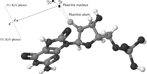
Figure 9.1 A schematic depiction of the decay process by which a fluorine-18 nucleus leads to the production of two high-energy photons (drawing not to scale).
One procedure used in neuroimaging involves injecting labeled FDG into the bloodstream and waiting about half an hour so that the FDG not used by neurons leaves the brain. The labeled FDG that remains in the brain tissues has been metabolically trapped within the tissue, and its concentration gives an indication of the regions of the brain that were active during that time. Therefore, the distribution of FDG in brain tissue, measured by the number of observed positron decays, can be a good indicator of the level of glucose metabolism, a proxy for neuronal activity. However, the time scales involved are not useful for studying brain activity related to changes in mental processes lasting only a few seconds.
However, the BOLD effect can be used in PET to obtain evidence of brain activity with higher temporal resolution. Other isotopes with half-lives shorter than that of FDG—among them carbon-11 (half-life 20 minutes), nitrogen-13 (half-life 10 minutes), and oxygen-15 (half-life 122 seconds) are used, integrated into a large number of different active molecules. The use of short-lived isotopes requires that a cyclotron be nearby to generate the unstable isotope so that it can be used before a significant fraction decays.
Despite the relevance of the previous techniques, the technique most commonly used today to study macro-scale brain behavior is magnetic-resonance imaging. Paul Lauterbur of the State University of New York at Stony Brook developed the theory behind MRI (Lauterbur 1973), building on previous work by Raymond Damadian and Herman Carr.
MRI is based on a physical phenomenon that happens when hydrogen nuclei are exposed to electric and magnetic fields. Hydrogen nuclei, which are in fact protons, have an intrinsic property, called nuclear spin, that makes them behave like small magnets that align themselves parallel to an applied magnetic field. When such a field is applied, a small fraction of the nuclei of atoms of hydrogen present, mostly in water molecules, align with the applied field. They converge to that alignment after going through a decaying oscillation of a certain frequency, called the resonating frequency, which depends on the intensity of the field. For a magnetic field of one tesla (T), the resonating frequency is 42 megahertz and it increases linearly with the strength of the field. Existing equipment used for human body imaging works with very strong magnetic fields (between 1.5 and 7 teslas). For comparison, the strength of the Earth’s magnetic field at sea level ranges from 25 to 65 microteslas, a value smaller by a factor of about 100,000.
If one applies a radio wave of a frequency close enough to the resonating frequency of these nuclei, the alignment deviates from the applied magnetic field, much as a compass needle would deviate from the north-south line if small pushes of the right frequency were to be applied in rapid succession. When this excitation process terminates, the nuclei realign themselves with the magnetic field, again oscillating at their specific resonating frequency. While doing this, they emit radio waves that can be detected and processed by computer and then used to create a three-dimensional image in which different types of tissues can be distinguished by their structure and their water content.
In practice, it isn’t possible to detect with precision the position of an atom oscillating at 42 megahertz, or some frequency of the same order, because the length of the radio waves emitted is too long. Because of physical limitations, we can only detect the source of a radio wave with an uncertainty on the order of its wavelength, which is, for the radio waves we are considering here, several meters. However, by modulating the magnetic field and changing its strength with time and along the different dimensions of space, the oscillating frequency of the atoms can be finely controlled to depend on their specific positions. This modulation causes each nucleus to emit at a specific frequency that varies with its location, and also with time, in effect revealing its whereabouts to the detectors. Figure 9.2 illustrates how control of the magnetic field can be used to pinpoint the locations of oscillating hydrogen nuclei.
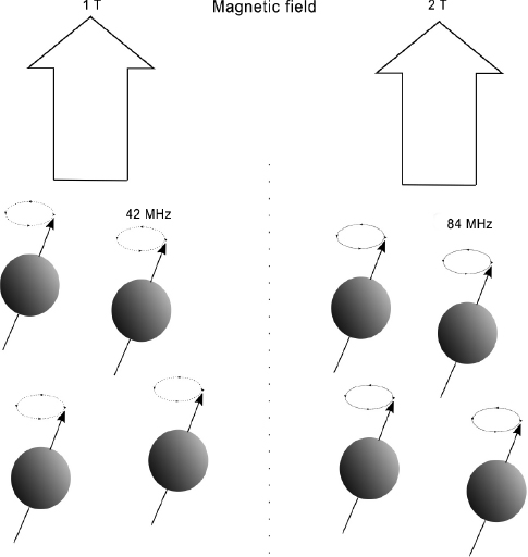
Figure 9.2 An illustration of how protons, oscillating at frequencies that depend on the strength of the magnetic field, make it possible to determine the precise locations of hydrogen atoms.
MRI has some limitations in terms of its space and time resolution. Because a strong enough signal must be obtained, the voxels cannot be too small. The stronger the magnetic field, the smaller the voxels can be, but even 7-tesla MRI machines cannot obtain high-quality images with voxels much smaller than about one cubic millimeter. However, as technology evolves, one can hope that this resolution will improve, enabling MRI to obtain images with significantly smaller voxels.
The physical principles underlying MRI can be used in accordance with many different protocols to obtain different sorts of information. In its simplest and most commonly used form, MRI is used to obtain static images of the brain for the purpose of diagnosing tumors or other diseases, which manifest themselves as changes in the brain’s macro-structures. These changes become visible because different tissues have different MRI signatures. Figure 9.3 shows the images of three slices of one brain. Image a corresponds to a slice near the top of the skull, with the cortex folds clearly visible. Image b shows some additional cortex folds; also visible are the lateral ventricles, where cerebrospinal fluid is produced, and the corpus callosum, the largest white matter structure in the brain. Image c shows a clearly abnormal structure (a benign brain tumor) on the right side of the image, near the center.
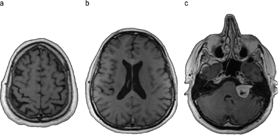
Figure 9.3 Images of brain slices obtained with magnetic-resonance imaging.
MRI techniques can also be used to obtain additional information about brain behavior and structure. Two important techniques are functional MRI and diffusion MRI.
In recent decades, functional MRI (fMRI) has been extensively used in brain research. Functional MRI was first proposed in 1991 by Jack Belliveau, who was working at the Athinoula A. Martinos Center, in Boston. (See Belliveau et al. 1991.) Belliveau used a contrast agent injected in the bloodstream to obtain a signal that could be correlated with the levels of brain activity in particular areas. In 1992, Kenneth Kwong (Martinos Center), Seiji Ogawa (AT&T Bell Laboratories), and Peter Bandettini (Medical College of Wisconsin) reported that the BOLD signal could be used directly in fMRI as a proxy for brain activity.
The BOLD effect can be used in fMRI because the difference in the magnetic properties of oxygen-rich and oxygen-poor hemoglobin leads to differences in the magnetic-resonance signals of oxygenated and deoxygenated blood. The magnetic resonance is stronger where blood is more highly oxygenated and weaker where it is not. The time scales involved in the BOLD effect largely define the temporal resolution. For fMRI, the hemodynamic response lasts more than 10 seconds, rising rapidly, peaking at 4 to 6 seconds, and then falling exponentially fast. The signal detected by fMRI lags the neuronal events triggering it by a second or two, because it takes that long for the vascular system to respond to the neuron’s need for glucose.
The time resolution of fMRI is sufficient for studying a number of brain processes. Neuronal activities take anywhere from 100 milliseconds to a few seconds. Higher reasoning activities, such as reading or talking, may take anywhere from a few seconds to many minutes. With a time resolution of a few seconds, most fMRI experiments study brain processes lasting from a few seconds to minutes, but because of the need for repetition, required to improve the signal-to-noise ratio, the experiments may last anywhere from a significant fraction of an hour to several hours,.
Diffusion MRI (dMRI) is another method that produces magnetic-resonance images of the structure of biological tissues. In this case, the images represent the local characteristics of molecular diffusion, generally of molecules of water (Hagmann et al. 2006). Diffusion MRI was first proposed, by Denis Le Bihan, in 1985. The technique is based on the fact that MRI can be made sensitive to the motion of molecules, so that it can be used to show contrast related to the structure of the tissues at microscopic level (Le Bihan and Breton 1985). Two specific techniques used in dMRI are diffusion weighted imaging (DWI) and diffusion tensor imaging (DTI).
Diffusion weighted imaging obtains images whose intensity correlates with the random Brownian motion of water molecules within a voxel of tissue. Although the relationship between tissue anatomy and diffusion is complex, denser cellular tissues tend to exhibit lower diffusion coefficients, and thus DWI can be used to detect certain types of tumors and other tissue malformations.
Tissue organization at the cellular level also affects molecule diffusion. The structural organization of the white matter of the brain (composed mainly of glial cells and of myelinated axons, which transmit signals from one region of the brain to another) can be studied in some detail by means of diffusion MRI because diffusion of water molecules takes places preferentially in some directions. Bundles of axons make the water diffuse preferentially in a direction parallel to the direction of the fibers.
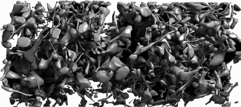
Diffusion tensor imaging uses the restricted directions of diffusion of water in neural tissue to produce images of neural tracts. In DTI, to each voxel corresponds one ellipsoid, whose dimensions give the intensity and the directions of the diffusion in the voxel. The ellipsoid can be characterized by a matrix (a tensor). The directional information at each voxel can be used to identify neural tracts. By a process called tractography, DTI data can be used to represent neural tracts graphically. By color coding individual tracts, it is possible to obtain beautiful and highly informative images of the most important connections between brain regions.
Tractography is used to obtain large-scale, low-resolution information about the connection patterns of the human brain. Figure 9.4 shows an image obtained by means of diffusion tensor imaging of the mid-sagittal plane, the plane that divides the brain into a left and a right side. The axon fibers connecting different regions of the brain, including the fibers in the corpus callosum connecting the two hemispheres and crossing the mid-sagittal plane, are clearly visible.
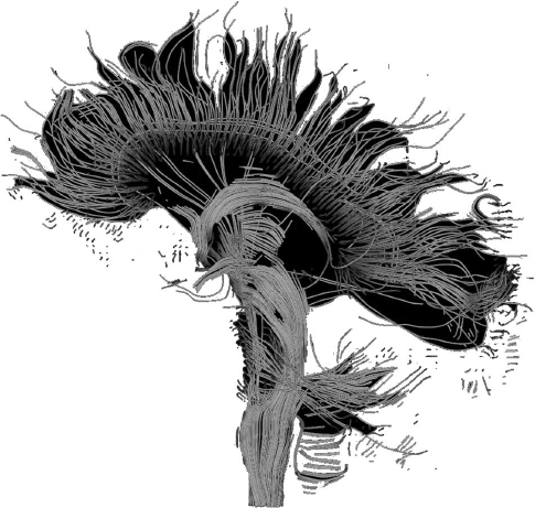
Figure 9.4 DTI reconstruction of tracts of brain fiber that run through the mid-sagittal plane. Image by Thomas Schultz (2006), available at Wikimedia Commons.
Electroencephalography (EEG) and magnetoencephalography (MEG) are two techniques that obtain information about brain behavior from physical principles different from the methods discussed above. Both EEG and MEG measure the activity level of neurons directly by looking how that activity affects electromagnetic fields.
When large groups of neurons fire in a coordinated way, they generate electric and magnetic fields that can be detected. The phenomenon, discovered in animals, was first reported by Richard Caton, a Liverpool physician (Caton 1875). In 1924, Hans Berger, inventor of the technique now known as EEG, recorded the first human electroencephalogram. (See Berger 1929.)
EEG works by recording the brain’s electrical activity over some period of time from multiple electrodes, generally placed on the scalp. The electric potential generated by the activity of an individual neuron is far too small to be picked up by the electrodes. EEG activity, therefore, reflects the contribution of the correlated activity of many neurons with related behavior and similar spatial orientation. Pyramidal neurons in the cortex produce the largest part of a scalp-recorded EEG signal because they are well aligned and because they fire in a highly correlated way. Because electric fields fall off with the square of the distance, activity from deeper structures in the brain is more difficult to detect.
The most common analyses performed on EEG signals are related to clinical detection of dysfunctional behaviors of the brain, which become visible in EEG signals as abnormal patterns. However, EEG is also used in brain research. Its spatial resolution is very poor, since the origin of the signals can’t be located more precisely than within a few centimeters. However, its time resolution is very good (on the order of milliseconds). EEG is sometimes used in combination with another imaging technique, such as MRI or PET.
In a related procedure known as electrocorticography (ECoG) or intracranial EEG (iEEG), electrodes are placed directly on the exposed surface of the brain to record electrical activity from the cerebral cortex. Since it requires removing a part of the skull to expose the brain’s surface, ECoG is not widely used in fundamental brain research with healthy human subjects, although it is extensively used in research with animals.
Magnetoencephalography (MEG), first proposed by David Cohen (1968), also works by detecting the effects in the electromagnetic fields of firing neurons, but in MEG the detectors are very sensitive magnetometers. To reduce the magnetic background noise, Cohen used a magnetically shielded room. (See figure 9.5.)
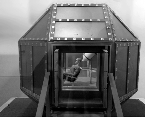
Figure 9.5 A model of the magnetically shielded room built by David Cohen in 1969 at MIT for the first magnetoencephalography experiments. Photo taken at Athinoula A. Martinos Center for Biomedical Imaging.
Whereas EEG detects changes in the electric field caused by ion flows, MEG detects tiny changes in the magnetic field caused by the intra-neuron and extra-neuron currents that occur in the correlated firing of large numbers of neurons (Okada 1983). Since currents must have similar orientations to generate magnetic fields that reinforce one another, it is again (as in EEG) the layer of pyramidal cells, which are situated perpendicular to the cortical surface, that produce the most easily measurable signals. Bundles of neurons with an orientation tangential to the scalp’s surface project significant portions of their magnetic fields outside the head. Because these bundles are typically located in the sulci, MEG is more useful than EEG for measuring neural activity in those regions, whereas EEG is more sensitive to neural activity generated on top of the cortical sulci, near the skull.
MEG and EEG both measure the perturbations in the electromagnetic field caused by currents inside the neurons and across neuron cell walls, but they differ greatly in the technology they use to do so. Whereas EEG uses relatively cheap electrodes placed on the skull, each connected to one amplifier, MEG uses arrays of expensive, highly sensitive magnetic detectors called superconducting quantum interference devices (SQUIDS). An MEG detector costs several million dollars to install and is very expensive to operate. Not only are the sensors very expensive; in addition, they must be heavily shielded from external magnetic fields, and they must be cooled to ultra-low temperatures. Efforts are under way to develop sensitive magnetic detectors that don’t have to be cooled to such low temperatures. New technologies may someday make it possible to place magnetic detectors closer to the skull and to improve the spatial resolution of MEG.
A recently developed method known as event-related optical signal (EROS) uses the fact that changes in brain-tissue activity lead to different light-scattering properties. These changes may be due to volumetric changes associated with movement of ions and water inside the neurons and to changes in ion concentration that change the diffraction index of the water in those neurons (Gratton and Fabiani 2001). Unlike the BOLD effect, these changes in the way light is scattered take place while the neurons are active and are spatially well localized. The spatial resolution of EROS is only slightly inferior to that of MRI, but its temporal resolution is much higher (on the order of 100 milliseconds). However, at present EROS is applicable only to regions of the cortex no more than a few centimeters away from the brain’s surface.
The techniques described in this section have been extensively used to study the behavior of working brains, and to derive maps of activity that provide significant information about brain processes, at the macro level. Whole-brain MRI analysis has enabled researchers to classify the voxels in a working brain into several categories in accordance with the role played by the neurons in each voxel (Fischl et al. 2002; Heckemann et al. 2006). Most studies work with voxels on the order of a cubic millimeter, which is also near the resolution level of existing MRI equipment. Many efforts aimed at making it possible to integrate imaging data from different subjects, and a number of atlases of the human brain have been developed—for example, the Probabilistic Atlas and Reference System for the Human Brain (Mazziotta et al. 2001) and the BigBrain Atlas (developed in the context of the Human Brain Project).
Integration of different techniques, including MRI, EEG, PET, and EROS, may lead to an improvement of the quality of the information retrieved. Such integration is currently a topic of active research.
A recently developed technique that shows a lot of promise to advance our understanding of brain function is optogenetics. In 1979, Francis Crick suggested that major advances in brain sciences would require a method for controlling the behavior of some individual brain cells while leaving the behavior of other brain cells unchanged. Although it is possible to electrically stimulate individual neurons using very thin probes, such a method does not scale to the study of large numbers of neurons. Neither drugs nor electromagnetic signals generated outside the brain are selective enough to target individual neurons, but optogenetics promises to be. Optogenetics uses proteins that behave as light-controlled membrane channels to control the activity of neurons. These proteins were known to exist in unicellular algae, but early in the twenty-first century researchers reported that they could behave as neuron membrane channels (Zemelman et al. 2002; Nagel et al. 2003) and could be used to stimulate or repress the activity of individual neurons or of smalls groups of neurons, both in culture (Boyden et al. 2005) and in live animals (Nagel et al. 2005). By using light to stimulate specific groups of neurons, the effects of the activity of these neurons on the behavior of the organism can be studied in great detail.
Optogenetics uses the technology of genetic engineering to insert into brain cells the genes that correspond to the light-sensitive proteins. Once these proteins are present in the cells of modified model organisms, light of the appropriate frequency can be used to stimulate neurons in a particular region. Furthermore, the activity of these neurons can be controlled very precisely, within milliseconds, by switching on and off the controlling light. Live animals, such as mice or flies, can be instrumented in this way, and the behaviors of their brains can then be controlled in such a way as to further our understanding of brain circuitry.
Optogenetics is not, strictly speaking, an imaging technique, but it can be used to obtain detailed information about brain behavior in live organisms with a resolution that cannot be matched by any existing imaging technique.