APPENDIX

Constructing Your Own Fourfold Tables

As we think about sound medical reasoning, we are often faced with diseases that are so rare that even a positive test doesn’t mean you have the disease. Many pharmaceutical products have such a low chance of their working that the risk of side effects is many times greater than the promise of a benefit.

The fourfold table allows us to easily calculate Bayesian probability models, such as the answer to the question “What is the probability that I have a disease, given that I already tested positive for it?” or “What is the probability that this medicine will help me, given that I have this symptom?”

Here I’ll use the example from Chapter 6 of the fictitious disease blurritis. Recall the information given:

• You took a blood test that came back positive for the hypothetical disease blurritis.
• The base rate for blurritis is 1 in 10,000, or .0001.
• The use of the hypothetical drug chlorohydroxelene ends in an unwanted side effect 5% of the time, or .05.
• The blood test for blurritus is wrong 2% of the time, or .02.

The question is, Should you take the medicine or not?

We start by drawing the table and labeling the rows and columns.

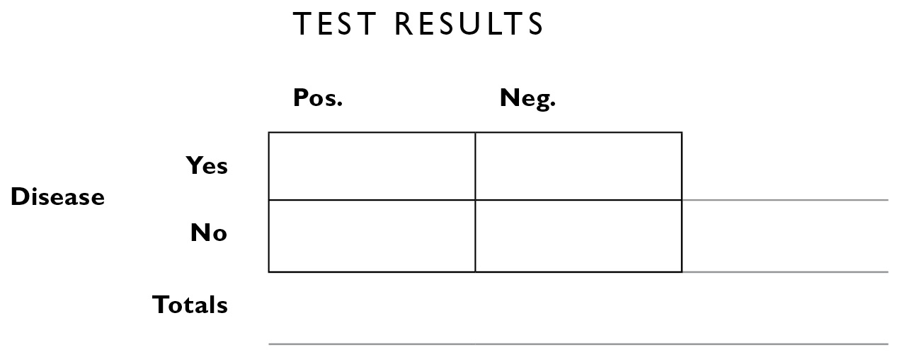
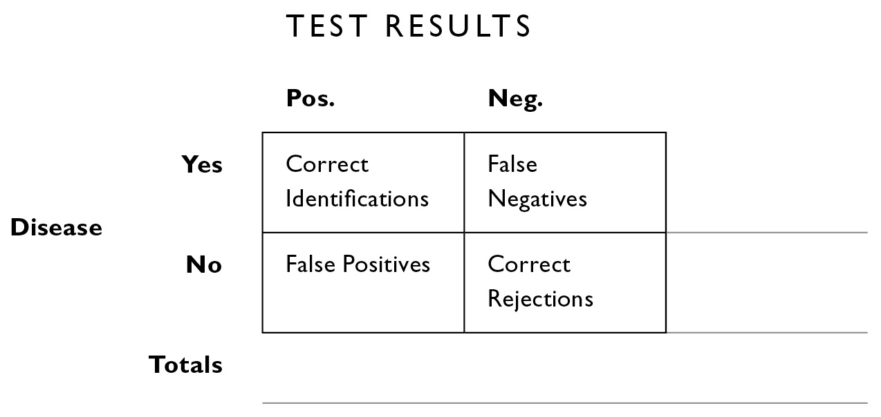
The boxes inside allow us to apportion the data into four mutually exclusive categories:

• people who have the disease who test positive (upper left interior box). We call these CORRECT IDENTIFICATIONS.
• people who have the disease who test negative (upper right interior box). We call these MISSES or FALSE NEGATIVES.
• people who don’t have the disease who test positive (lower left interior box). We call these FALSE POSITIVES.
• people who don’t have the disease who test negative (lower right interior box). We call these CORRECT REJECTIONS.

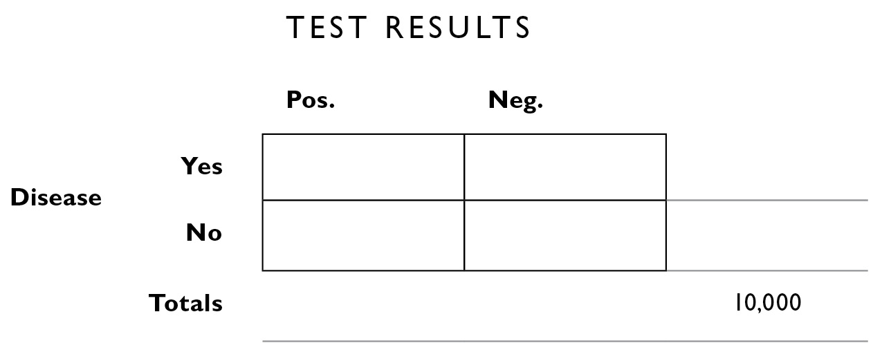
Now we start filling in what we know. The base rate of the disease is 1 in 10,000. In the lower right corner, outside the big box, I’ll fill in the “grand total” of 10,000. I call this the population box because it is the number that tells us how many there are in the total population we’re looking at (we could fill in 320 million for the population of the United States here, and then work with the total number of cases reported per year—32,000—but I prefer filling in the smaller numbers of the “incident rate” because they’re easier to work with).

What we seek to calculate, with the help of this table, are the numbers in the other boxes, both the boxes inside the outlines and the boxes outside. Of those 10,000 people, we know 1 of them has blurritis. We don’t know yet how that person is apportioned by test results, so we fill in the number 1 all the way to the right, corresponding to “Disease: Yes.”

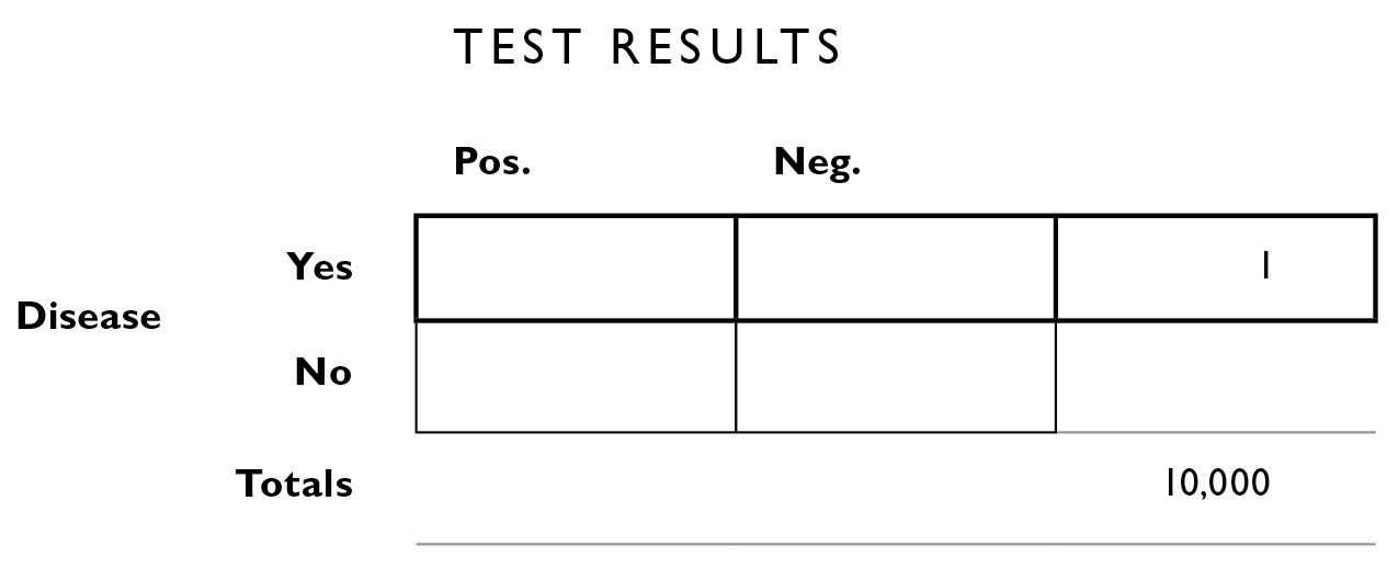
The way the table is designed, numbers from top to bottom and from left to right are supposed to add up to their “marginal totals” along the outskirts of the figure. This is logical: If the number of people with the disease = 1, and the total number of people under consideration is 10,000, we know the number of people who do not have the disease within this population must be: 10,000−1 = 9,999. So we can fill that in the table next.

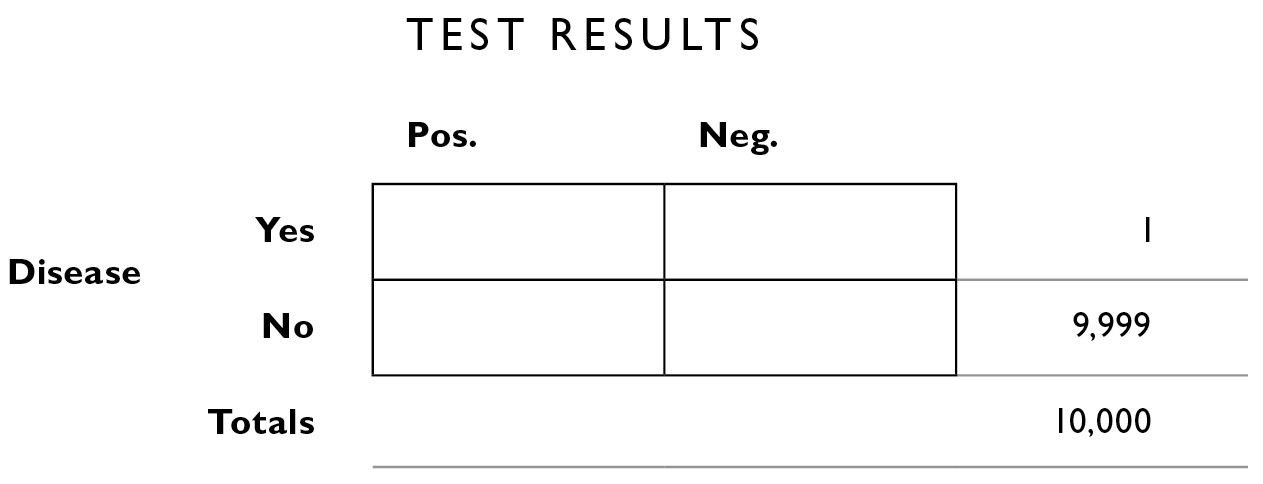
We know from what the doctor told us (above) that 2% of the time, the test is inaccurate. We apply that 2% figure to the totals along the right margin. Of the 9,999 who do not have the disease, 2% of them will be given the wrong diagnosis. That is, although they don’t have the disease, the test will say they do (a false positive, the lower left interior box). We calculate 2% × 9,999 = 199.98, and round that to 200.

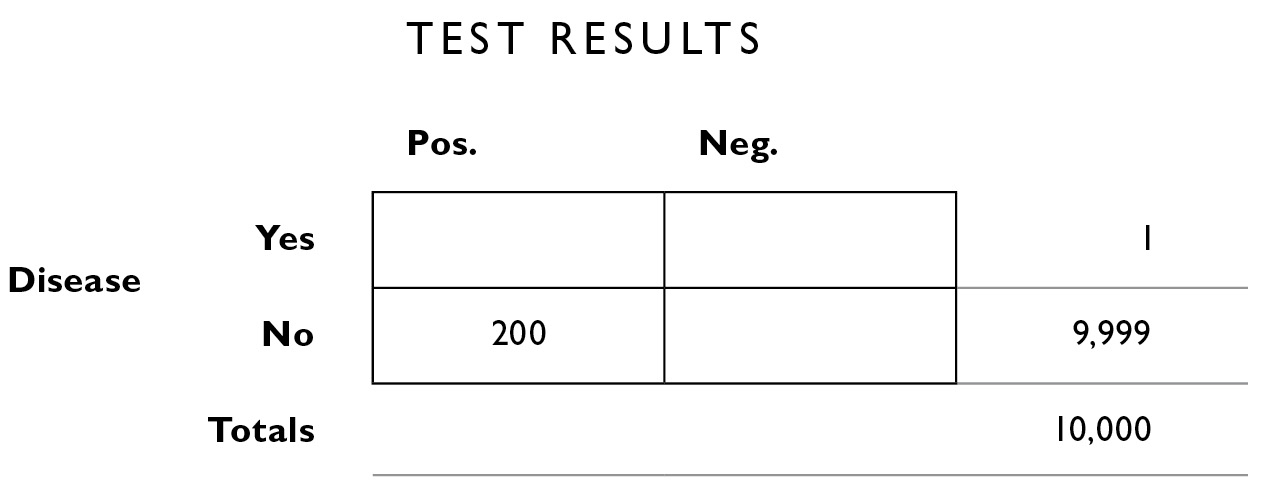
Now, because the numbers need to add up in rows and columns, we can calculate the number of people who don’t have the disease and whose test results are negative—the correct rejections. This is 9,999−200 = 9,799.

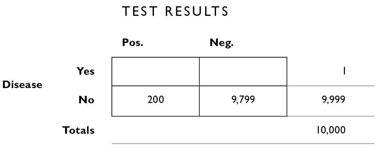
Now we fill in the other misdiagnoses, the 2% false negatives. False negative means you have the disease and the test says you don’t—they’re in the upper right interior box. Only 1 person has the disease (as we see in the far right margin). We calculate 2% × 1 = .02, or 0 if you round.

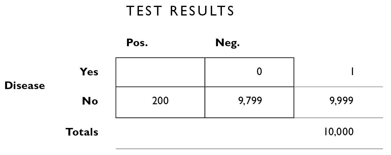
And of course that lets us fill in the empty square with 1 (we get that by starting with the margin total, 1, and subtracting the 0 in the top right box, to fill in the empty box on the top left—remember, the numbers need to add up in every row and every column).

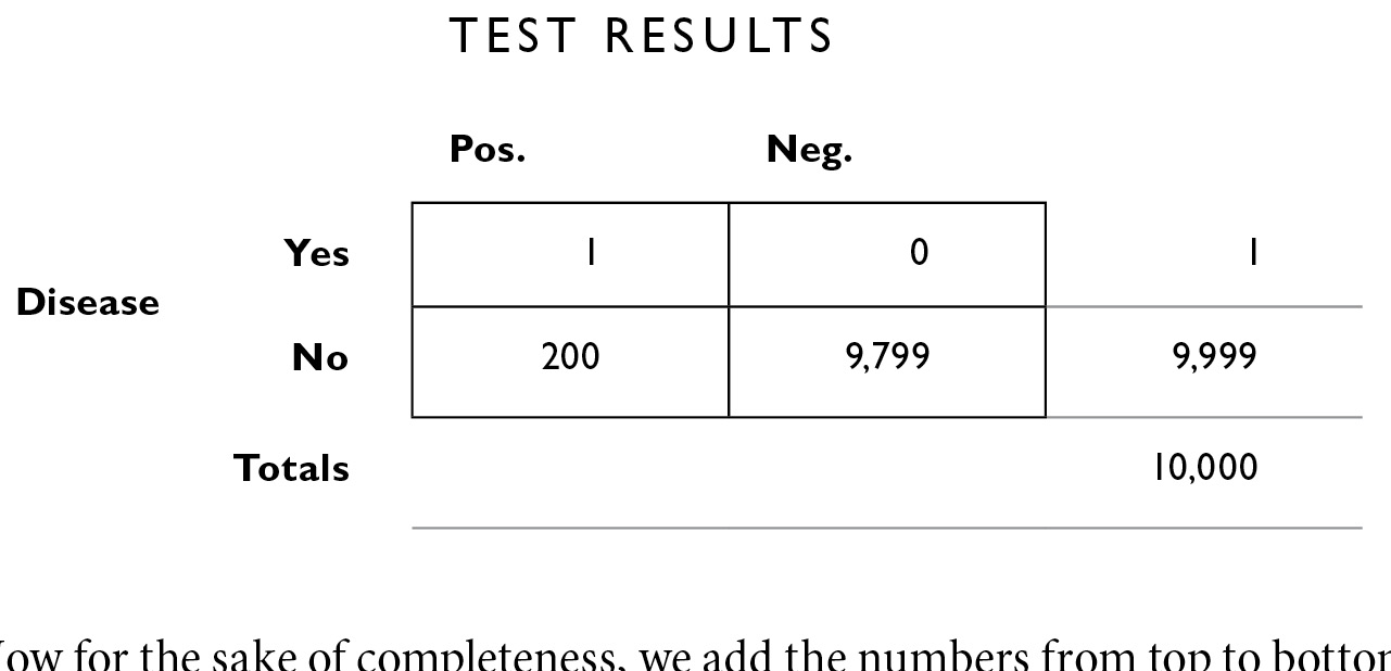
Now for the sake of completeness, we add the numbers from top to bottom to fill in the margins on the bottom outside the table—the total number of people who got positive test results is simply the sum of those in that column: 1 + 200 = 201. And the total number of people who got negative results is 0 + 9,799 = 9,799.

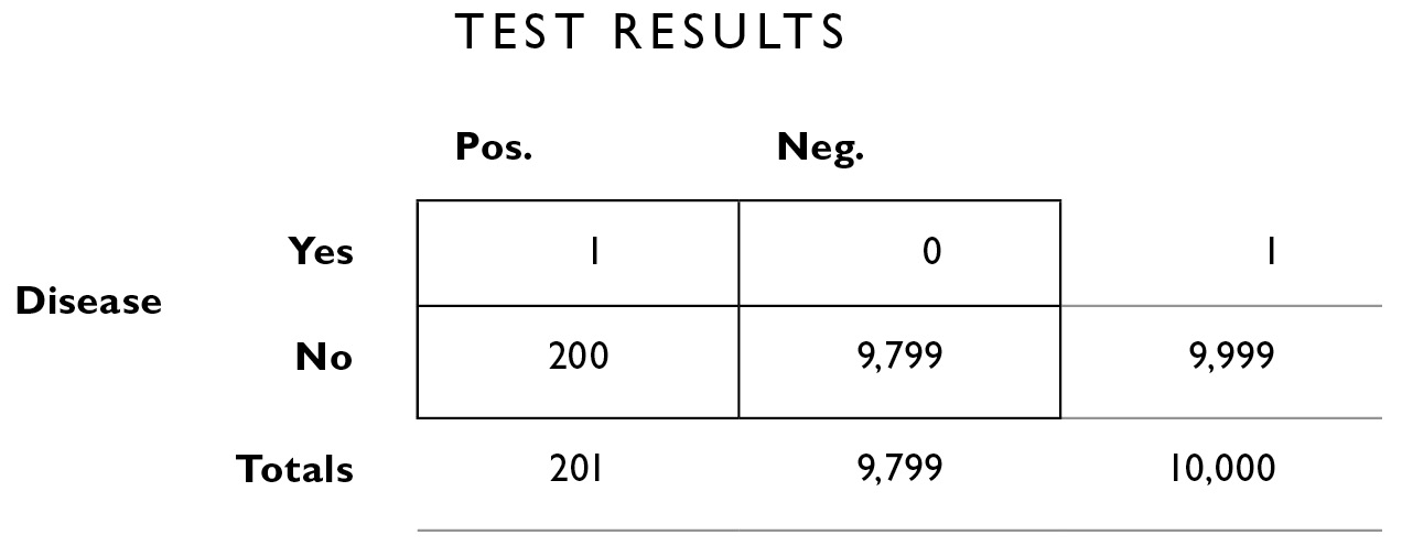
From here, we can solve the problems as shown in Chapter 6.

1. What is the probability that you have the disease, given that you tested positive?

We traditionally replace the word given with the symbol | and the word probability with the letter p to construct a kind of equation that looks like this:

1.1. p(You have the disease | you tested positive)

This format is convenient because it reminds us that the first part of the sentence—everything before the | symbol, becomes the numerator (top part) of a fraction, and everything after the | symbol becomes the denominator.

To answer question 1, we look only at the column of people with positive test results, the left column. There is 1 person who actually has the disease out of 201 who tested positive. The answer to question 1 is 1/201, or .49%.

2. What is the probability that you will test positive, given that you have the disease?

2.1. p(You test positive | you have the disease)

Here we look only at the top row, and construct the fraction 1/1 to conclude that there is 100% chance that you’ll test positive if you really and truly have the disease.

Remember that my hypothetical treatment, chlorohydroxelene, has a 20% chance of side effects. If we treat everyone who tested positive for blurritis—all 201 of them—20%, or 40, will experience the side effect. Remember, only 1 person actually has the disease, so the treatment is 40 times more likely to provide side effects than a cure.

In these two cases I described in Chapter 6, blurritis and the blue face disease, even if you tested positive for them, it is unlikely you have the disease. Of course, if you really have the disease, choosing the right drug is important. What can you do?

You can take the test twice. We apply the multiplicative law of probability here, assuming that the results of the tests are independent. That is, whatever errors might cause you of all people to get an incorrect result are random—it’s not as though someone at the testing lab has it in for you—and so if you got an incorrect result once, you’re not any more likely to get an incorrect result again than anyone else would be. Recall that I said the test had a 2% chance of being wrong. The probability of its being wrong twice in a row is 2% × 2%, or .0004. If you prefer to work with fractions, the probability was 1/50, and 1/50 × 1/50 = 1/2500. But even this statistic doesn’t take into account the base rate, the rarity of the disease. And doing that is the whole point of this section.

The helpful thing to do, of course, is to construct a fourfold table to answer the question “What is the probability that I have the disease, given that I tested positive for it twice in a row?”

When we started looking at blurritis, we had just a bunch of numbers and we placed them into a fourfold table; this allowed us to easily calculate our updated probabilities. One of the features of Bayesian inferencing is that you can place those updated probabilities into a new table to update again. With each new update of information, you can build a new table and home in on more and more accurate estimates.

The table looked like this when it was all filled in:

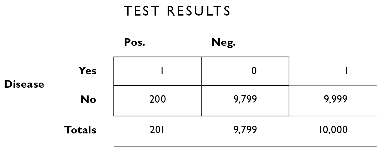
and we read off the following from the table:

Number of people who tested positive: 201

Number of people who tested positive and have the disease: 1

Number of people who tested positive and don’t have the disease: 200

Notice that now we’re looking only at half the table, the half for people with positive test results. This is because the question we want to answer assumes you tested positive: “What is the probability that I actually have the disease if I test positive for it twice in a row?”

So now we construct a new table using this information. For the table headings, the second test result can be positive or negative, you can have or not have the disease, and we’re no longer looking at the total population of 10,000; we’re looking only at that subset of the 10,000 who tested positive the first time: 201 people. So we put 201 in the population box on the lower right margin.

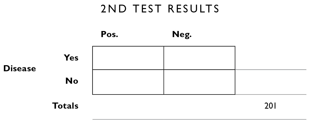
We can also fill in some of the additional information from up above. We know the number of people in this population who do and don’t have the disease and so we fill those in on the right margin.

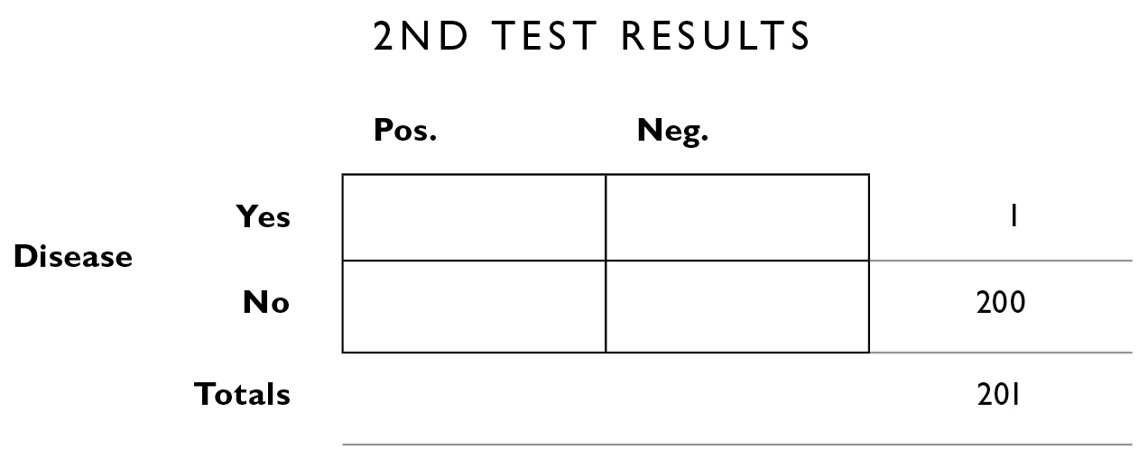
Now we go back to the original information we were given, that the test makes errors 2% of the time. One person actually has the disease; 2% of the time, it will be incorrectly diagnosed, and 98%, it will be correctly diagnosed: 2% of 1 = .02. I’ll round that down to 0—this is the number of people who show false negatives (they have the disease, but it was incorrectly diagnosed the second time). And 98% of 1 is close to 1.

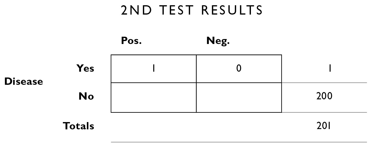
Next we apply the same 2% error rate to the people who don’t have the disease. 2% of the 200 who don’t have the disease will test positive (even though they’re healthy): 2% of 200 = 4. That leaves 196 for the correctly diagnosed interior box in the lower right.

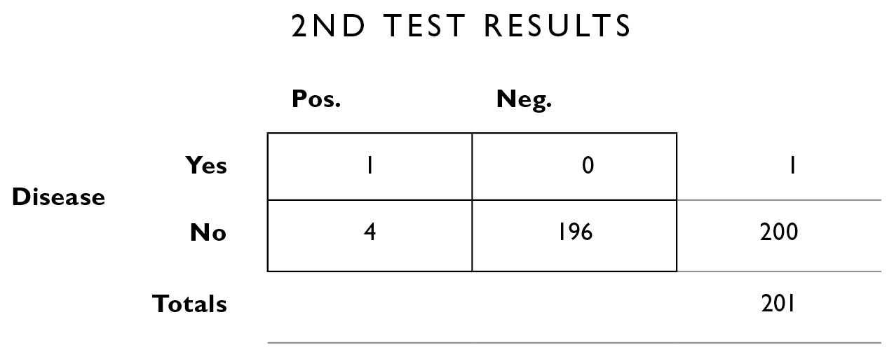
We can add up the columns vertically to obtain the marginal totals, which we’ll need to compute our new updated probabilities.

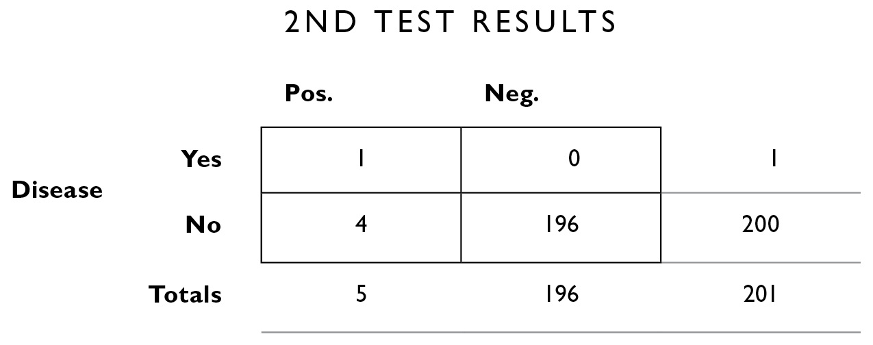
As before, we calculate on the left column, because we’re interested only in those people who tested positive a second time.

Of the 5 people who tested positive a second time, 1 actually has the disease: 1/5 = .20. In other words, the disease is sufficiently rare that even if you test positive twice in a row, there is still only a 20% chance you have it, and therefore an 80% chance you don’t.

What about those side effects? If we start everyone who tested positive twice in a row on my fictitious chlorohydroxelene with the 5% side effects, 5% of those 5 people, or .25, will experience side effects. So although it’s unlikely you have the disease, it’s also unlikely all your hair will fall out. For every 5 people who take the treatment, 1 will be cured (because that person actually has the disease) and .25 will have the side effects. In this case, with two tests, you’re now about 4 times more likely to experience the cure than the side effects, a nice reversal of what we saw before. (If it makes you uncomfortable to talk about .25 of a person, just multiply all the numbers above by 4.)

We can take Bayesian statistics a step further. Suppose a newly published study shows that if you are a woman, you’re ten times more likely to get the disease than if you’re a man. You can construct a new table to take this information into account, and to refine the estimate that you actually have the disease.

The calculations of probabilities in real life have applications far beyond medical matters. I asked Steve Wynn, who owns five casinos (at his Wynn and Encore hotels in Las Vegas, and the Wynn, Encore, and Palace in Macau), “Doesn’t it hurt, just a little, to see customers walking away with large pots of your money?”

“I’m always happy to see people win. It creates a lot of excitement in the casino.”

“Come on, really? It’s your money. Sometimes people walk away with millions.”

“First of all, you know we make a lot more than we pay out. Second, we usually get the money back. In all these years, I’ve never seen a big winner actually walk away. They come back to the casino and play with what they won, and we usually get it all back. The reason they’re there in the first place is that, like most people with a self-indulgence such as golf or fine wine, they like the game more than the money. Winning provides them with capital for the game, without them having to write a check. People lose at 100 cents on the dollar, they win at 99 cents on the dollar. That 1% is our margin.”

The expected value of a casino bet always favors the house. Now, there is a psychology of gambling that leads winners who could walk away with a fortune to stay and lose it all. Setting this aside, even if all the winners did walk away, the long-run odds are still in favor of the house. Which leads us to extended warranties on things like laser printers, computers, vacuum cleaners, and DVD players. The big discount retailers really push these warranties, and they play upon your quite reasonable reluctance to pay big repair bills on an item you just bought. They promise “worry-free” repairs at a premium price. But make no mistake—this is not a service offered out of the retailer’s generosity, but as a moneymaking enterprise. For many retailers, the real profits are not in selling you the initial item but in selling you the warranty to protect it.

Such warranties are almost always a bad deal for you and a good deal for “the house.” If there is a 10% chance that you’ll use it, and it will save you $300 in repair costs, then its expected value is $30. If they’re charging you $90 for it, that $60 above the expected value is a sure profit for the retailer. They try to suck you in with pleas like “If this breaks, the minimum repair charge will be two hundred dollars. The warranty only costs ninety dollars, so you’re coming out way ahead.” But don’t be taken in. You only come out ahead if you’re one of those 10% who needs it. The rest of the time, they come out ahead. Medical decision-making is no different. You can apply expected value calculations to the costs and benefits of various treatment options. There exist strictly mathematical methods for calculating these values of course—there is nothing magic about using these contingency tables. Many people prefer them, though, because they act as a heuristic for organizing the information, and they allow for an easy visual display of the numbers, which in turn helps you to catch any errors you might have made along the way. In fact, much of the advice in this book about staying organized comes down to putting systems in place that will help us catch errors when we make them, or recover from the errors we inevitably all make.