Hash Tables

Introducing Hash Tables

Hash tables are excellent for quick storage and retrieval of data based on key-value pairs. In JavaScript, JavaScript objects work this way by defining a key (property) and its associated value. Figure 11-1 shows each key and its associated item.

../images/465726_1_En_11_Chapter/465726_1_En_11_Fig1_HTML.jpg — Figure 11-1
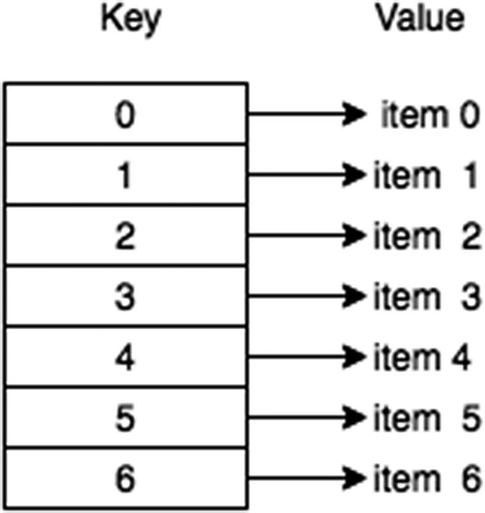
Simple hash table overview

A hash table contains two main functions: put() and get() . put() is used for storing data into the hash table, while get() is used for retrieving data from the hash table. Both of these functions have a time complexity of O(1).

In a nutshell, a hash table is analogous to an array whose index is calculated with a hashing function to identify a space in memory uniquely.

localStorage is an example of a data structure based on a hash table. It is a native JavaScript object supported by all major browsers. It lets developers persist data inside the browser, meaning it can be accessed after a session.

1 localStorage.setItem("testKey","testValue");

2 location = location; // refreshes the page

3

4 //-----------------------------------

5 localStorage.getItem("testKey"); // prints "testValue"

Hashing Techniques

The most important part of a hash table is the hash function. The hash function converts a specified key into an index for an array that stores all of the data. The three primary requirements for a good hash function are as follows:

Deterministic: Equal keys produce equal hash values.
Efficiency: It should be O(1) in time.
Uniform distribution: It makes the most use of the array.

The first technique for hashing is to use prime numbers. By using the modulus operator with prime numbers, a uniform distribution of the index can be guaranteed.

Prime Number Hashing

Prime numbers in hashing are important. This is because modulus division using prime numbers yields an array index in a distributed manner.

Modulus number: 11

4 % 11 = 4

7 % 11 = 7

9 % 11 = 9

15 % 11 = 4

Collisions can be seen with 15 and 4 yielding the same key; handling this collision is discussed later in this chapter. What is important here is that modulus by prime numbers guarantees the best distribution for a fixed size. Modulus by a small nonprime number such as 4 guarantees only a range from 0 to 3 and leads to a large number of collisions.

Modulus number: 4

6 % 4 = 2

10 % 4 = 2

This is the first hashing technique that will be observed. Take a look at Figure 11-2, which is a hash table with two arrays of size 11, and each of the 11 elements is empty. One array is for the keys, and the other is for values.

../images/465726_1_En_11_Chapter/465726_1_En_11_Fig2_HTML.jpg — Figure 11-2
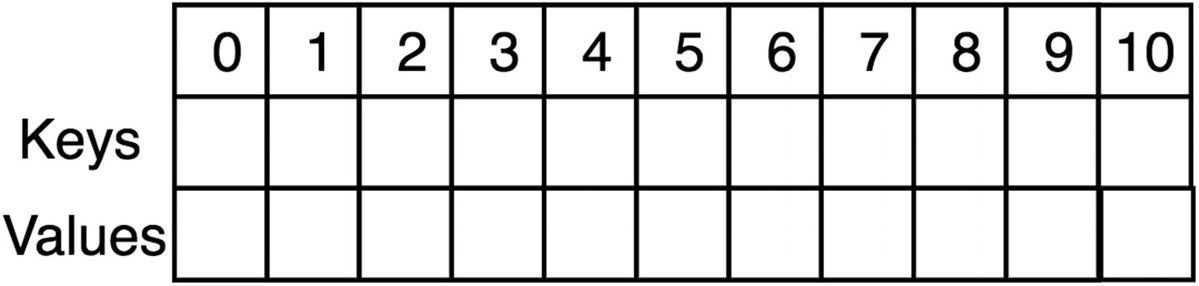
Hash table of size 11, with all empty elements

In this example, keys are integers, and strings are being stored as keys. Let’s hash the following key-value pairs:

{key:7, value: "hi"}

{key:24, value: "hello"}

{key:42, value: "sunny"}

{key:34, value: "weather"}

Prime number: 11

7 % 11 = 7

24 % 11 = 2

42 % 11 = 9

34 % 11 = 1

After all the key-value pairs have been inserted, the resulting hash table is shown in Figure 11-3.

../images/465726_1_En_11_Chapter/465726_1_En_11_Fig3_HTML.jpg — Figure 11-3
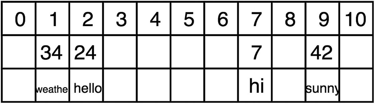
Hash table after inserting the value pairs

Now let’s hash {key:18, value: “wow”}.

Prime number: 11

18 % 11 = 7

This is a problem because 7 already exists in the index of 7 and causes an index collision. With a perfect hashing function, there are no collisions. However, collision-free hashing is almost impossible in most cases. Therefore, strategies for handling collisions are needed for hash tables.

Probing

To work around occurring collisions, the probing hashing technique finds the next available index in the array. The linear probing technique resolves conflicts by finding the next available index via incremental trials, while quadratic probing uses quadratic functions to generate incremental trials.

Linear Probing

Linear probing works by finding the next available index by incrementing one index at a time. For example, in the case of 18 and 7 hashing to the same key, 18 would be hashed into key 8 because that’s the next empty spot (see Figure 11-4).

../images/465726_1_En_11_Chapter/465726_1_En_11_Fig4_HTML.jpg — Figure 11-4
Hash table 1 after using linear probing

However, now when the get(key) function is used, it has to start at the original hash result (7) and then iterate until 18 is found.

The main disadvantage of linear probing is it easily creates clusters, which are bad because they create more data to iterate through.

Quadratic Probing

Quadratic probing is a good technique for addressing the cluster issue. Quadratic probing uses perfect squares instead of incrementing by 1 each time, and this helps to evenly distribute across the available indices, as shown in Figure 11-5.

h + (1)^2, h + (2)^2, h + (3)^2, h + (4)^2

h + 1, h + 4, h + 9, h + 16

../images/465726_1_En_11_Chapter/465726_1_En_11_Fig5_HTML.jpg — Figure 11-5
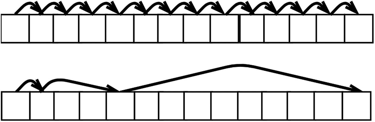
Linear probing (on top) and quadratic probing (on bottom)

Rehashing/Double-Hashing

Another great way to uniformly distribute the keys is by having a second hashing function that hashes the result from the original. These are the three primary requirements for a good second hash function:

Different: It needs to be different to distribute it better.
Efficiency: It should still be O(1) in time.
Nonzero: It should never evaluate to zero. Zero gives the initial hash value.

A commonly used second hashing function is as follows:

hash2(x) = R − (x % R)

Here, x is the result from hashing the first time, and R is less than the size of the hash table. Each hash collision is resolved by the following, where i is the iteration trial number:

i * hash₂(x)

Hash Table Implementation

Now that hash tables have been explained, let’s implement one from scratch. In this section, you will apply three different techniques to the same example. The following are the example key-value pairs that will be used:

7, “hi”
20, “hello”
33, “sunny”
46, “weather”
59, “wow”
72, “forty”
85, “happy”
98, “sad”

Using Linear Probing

Let’s start the example with simple linear probing.

1 function HashTable(size) {

2 this.size = size;

3 this.keys = this.initArray(size);

4 this.values = this.initArray(size);

5 this.limit = 0;

6 }

7

8 HashTable.prototype.put = function(key, value) {

9 if (this.limit >= this.size) throw 'hash table is full'

10

11 var hashedIndex = this.hash(key);

12

13 // Linear probing

14 while (this.keys[hashedIndex] != null) {

15 hashedIndex++;

16

17 hashedIndex = hashedIndex % this.size;

18

19 }

20

21 this.keys[hashedIndex] = key;

22 this.values[hashedIndex] = value;

23 this.limit++;

24 }

25

26 HashTable.prototype.get = function(key) {

27 var hashedIndex = this.hash(key);

28

29 while (this.keys[hashedIndex] != key) {

30 hashedIndex++;

31

32 hashedIndex = hashedIndex % this.size;

33

34 }

35 return this.values[hashedIndex];

36 }

37

38 HashTable.prototype.hash = function(key) {

39 // Check if int

40 if (!Number.isInteger(key)) throw 'must be int';

41 return key % this.size;

42 }

43

44 HashTable.prototype.initArray = function(size) {

45 var array = [];

46 for (var i = 0; i < size; i++) {

47 array.push(null);

48 }

49 return array;

50 }

51

52 var exampletable = new HashTable(13);

53 exampletable.put(7, "hi");

54 exampletable.put(20, "hello");

55 exampletable.put(33, "sunny");

56 exampletable.put(46, "weather");

57 exampletable.put(59, "wow");

58 exampletable.put(72, "forty");

59 exampletable.put(85, "happy");

60 exampletable.put(98, "sad");

Here is the result:

Keys:

[ 85, 98, null, null, null, null, null, 7, 20, 33, 46, 59, 72 ]

Values:

[ 'happy', 'sad', null, null, null, null, null, 'hi', 'hello', 'sunny', 'weather', 'wow', 'forty' ]

Using Quadratic Probing

Now, let’s change the put() and get() methods to use quadratic probing.

1 HashTable.prototype.put = function (key, value) {

2 if (this.limit >= this.size) throw 'hash table is full'

3

4 var hashedIndex = this.hash(key), squareIndex = 1;

5

6 // quadratic probing

7 while (this.keys[hashedIndex] != null) {

8 hashedIndex += Math.pow(squareIndex,2);

9

10 hashedIndex

11 squareIndex++;

12 }

13

14 this.keys[hashedIndex] = key;

15 this.values[hashedIndex] = value;

16 this.limit++;

17 }

18

19 HashTable.prototype.get = function (key) {

20 var hashedIndex = this.hash(key), squareIndex = 1;

21

22 while ( this.keys[hashedIndex] != key ) {

23 hashedIndex += Math.pow(squareIndex, 2);

24

25 hashedIndex = hashedIndex % this.size;

26 squareIndex++;

27 }

28

29 return this.values[hashedIndex];

30 }

Here is the result:

Keys:

[ null, null, null, 85, 72, null, 98, 7, 20, null, 59, 46, 33 ]

Values:

[ null, null, null, 'happy', 'forty', null, 'sad', 'hi', 'hello', null, 'wow', 'weather', 'sunny' ]

This result is more uniformly distributed than the result from linear probing. It would be easier to see with a bigger array size and more elements.

Using Double-Hashing with Linear Probing

Finally, let’s combine double-hashing and linear probing. Recall the common second hash function, hash₂(x) = R − (x % R), where x is the result from hashing the first time, and R is less than the size of the hash table.

1 HashTable.prototype.put = function(key, value) {

2 if (this.limit >= this.size) throw 'hash table is full'

3

4 var hashedIndex = this.hash(key);

5

6 while (this.keys[hashedIndex] != null) {

7 hashedIndex++;

8

9 hashedIndex = hashedIndex % this.size;

10

11 }

12 this.keys[hashedIndex] = key;

13 this.values[hashedIndex] = value;

14 this.limit++;

15 }

16

17 HashTable.prototype.get = function(key) {

18 var hashedIndex = this.hash(key);

19

20 while (this.keys[hashedIndex] != key) {

21 hashedIndex++;

22

23 hashedIndex = hashedIndex % this.size;

24

25 }

26 return this.values[hashedIndex];

27 }

28

29 HashTable.prototype.hash = function(key) {

30 if (!Number.isInteger(key)) throw 'must be int'; // check if int

31 return this.secondHash(key % this.size);

32 }

33

34 HashTable.prototype.secondHash = function(hashedKey) {

35 var R = this.size - 2;

36 return R - hashedKey % R;

37 }

Here is the result:

Keys:

[ null, 59, 20, 85, 98, 72, null, 7, null, 46, null, 33, null ]

Values:

[ null, 'wow', 'hello', 'happy', 'sad', 'forty', null, 'hi', null, 'weather', null, 'sunny', null ]

Again, double-hashing results in a more uniformly distributed array than the result from linear probing. Both quadratic probing and double-hashing are great techniques to reduce the number of collisions in a hash table. There are collision resolution algorithms far more advanced than these techniques, but they are beyond the scope of this book.

Summary

A hash table is a fixed-sized data structure in which the size is defined at the start. Hash tables are implemented using a hash function to generate an index for the array. A good hash function is deterministic, efficient, and uniformly distributive. Hash collisions should be minimized with a good uniformly distributive hash function, but having some collisions is unavoidable. Hash collision-handling techniques include but are not limited to linear probing (incrementing the index by 1), quadratic probing (using a quadratic function to increment the index), and double-hashing (using multiple hash functions).

The next chapter explores stacks and queues, which are dynamically sized data structures.

11. Hash Tables

Introducing Hash Tables

Hashing Techniques

Prime Number Hashing

Probing

Linear Probing

Quadratic Probing

Rehashing/Double-Hashing

Hash Table Implementation

Using Linear Probing

Using Quadratic Probing

Using Double-Hashing with Linear Probing

Summary