© Sammie Bae 2019

Sammie BaeJavaScript Data Structures and Algorithmshttps://doi.org/10.1007/978-1-4842-3988-9_1

1. Big-O Notation

Sammie Bae¹ 

(1)

Hamilton, ON, Canada

 

O(1) is holy.

—Hamid Tizhoosh

Before learning how to implement algorithms, you should understand how to analyze the effectiveness of them. This chapter will focus on the concept of Big-O notation for time and algorithmic space complexity analysis. By the end of this chapter, you will understand how to analyze an implementation of an algorithm with respect to both time (execution time) and space (memory consumed).

Big-O Notation Primer

The Big-O notation measures the worst-case complexity of an algorithm. In Big-O notation, n represents the number of inputs. The question asked with Big-O is the following: “What will happen as n approaches infinity?”

When you implement an algorithm, Big-O notation is important because it tells you how efficient the algorithm is. Figure 1-1 shows some common Big-O notations.

Figure 1-1

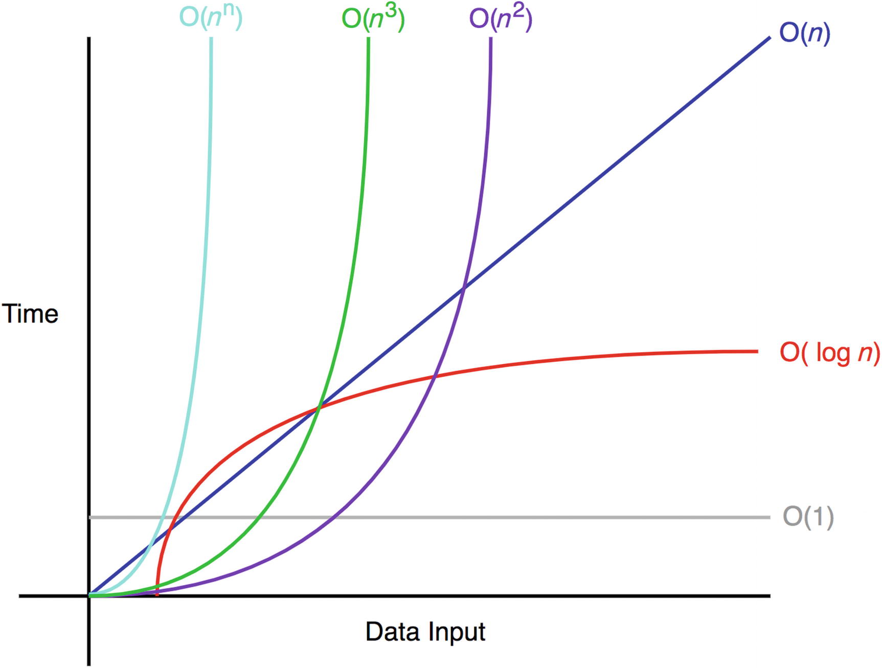
Common Big-O complexities

The following sections illustrate these common time complexities with some simple examples.

Common Examples

O(1) does not change with respect to input space. Hence, O(1) is referred to as being constant time. An example of an O(1) algorithm is accessing an item in the array by its index. O(n) is linear time and applies to algorithms that must do n operations in the worst-case scenario.

An example of an O(n) algorithm is printing numbers from 0 to n-1, as shown here:

1 function  exampleLinear(n) {

2                   for  (var  i = 0 ; i <  n; i++ ) {

3                              console.log(i);

4                   }

5  }

Similarly, O(n²) is quadratic time, and O(n³) is cubic time. Examples of these complexities are shown here:

1 function  exampleQuadratic(n) {

2                   for  (var  i = 0 ; i <  n; i++ ) {

3                                 console.log(i);

4                                for  (var  j =  i; j <  n; j++ ) {

5                                             console.log(j);

6                              }

7                   }

8  }

1 function  exampleCubic(n) {

2                   for  (var  i = 0 ; i <  n; i++ ) {

3                                  console.log(i);

4                                for  (var  j =  i; j <  n; j++ ) {

5                                              console.log(j);

6                                                  for  (var  k =  j; j <  n; j++ ) {

7                                                          console.log(k);

8                                                  }

9                                }

10           }

11 }

Finally, an example algorithm of logarithmic time complexity is printing elements that are a power of 2 between 2 and n. For example, exampleLogarithmic(10) will print the following:

2,4,8,16,32,64

The efficiency of logarithmic time complexities is apparent with large inputs such as a million items. Although n is a million, exampleLogarithmic will print only 19 items because log₂(1,000,000) = 19.9315686. The code that implements this logarithmic behavior is as follows:

1 function  exampleLogarithmic(n) {

2                   for  (var  i = 2 ; i <=  n; i= i*2 ) {

3                          console.log(i);

4                  }

5  }

Rules of Big-O Notation

Let’s represent an algorithm’s complexity as f(n). n represents the number of inputs, f(n)_time represents the time needed, and f(n)_space represents the space (additional memory) needed for the algorithm. The goal of algorithm analysis is to understand the algorithm’s efficiency by calculating f(n). However, it can be challenging to calculate f(n). Big-O notation provides some fundamental rules that help developers compute for f(n).

• Coefficient rule: If f(n) is O(g(n)), then kf(n) is O(g(n)), for any constant k > 0. The first rule is the coefficient rule, which eliminates coefficients not related to the input size, n. This is because as n approaches infinity, the other coefficient becomes negligible.

• Sum rule: If f(n) is O(h(n)) and g(n) is O(p(n)), then f(n)+g(n) is O(h(n)+p(n)). The sum rule simply states that if a resultant time complexity is a sum of two different time complexities, the resultant Big-O notation is also the sum of two different Big-O notations.

• Product rule: If f(n) is O(h(n)) and g(n) is O(p(n)), then f(n)g(n) is O(h(n)p(n)). Similarly, the product rule states that Big-O is multiplied when the time complexities are multiplied.

• Transitive rule: If f(n) is O(g(n)) and g(n) is O(h(n)), then f(n) is O(h(n)). The transitive rule is a simple way to state that the same time complexity has the same Big-O.

• Polynomial rule: If f(n) is a polynomial of degree k, then f(n) is O(n^k). Intuitively, the polynomial rule states that polynomial time complexities have Big-O of the same polynomial degree.

• Log of a power rule: log(nk) is O(log(n)) for any constant k > 0. With the log of a power rule, constants within a log function are also ignored in Big-O notation.

Special attention should be paid to the first three rules and the polynomial rule because they are the most commonly used. I’ll discuss each of those rules in the following sections.

Coefficient Rule: “Get Rid of Constants”

Let’s first review the coefficient rule . This rule is the easiest rule to understand. It simply requires you to ignore any non-input-size-related constants. Coefficients in Big-O are negligible with large input sizes. Therefore, this is the most important rule of Big-O notations.

• If f(n) is O(g(n)), then kf(n) is O(g(n)), for any constant k > 0.

This means that both 5f(n) and f(n) have the same Big-O notation of O(f(n)).

Here is an example of a code block with a time complexity of O(n):

1   function a(n){

2       var count =0;

3       for (var i=0;i<n;i++){

4           count+=1;

5       }

6       return count;

7   }

This block of code has f(n) = n. This is because it adds to countn times. Therefore, this function is O(n) in time complexity:

1   function a(n){

2       var count =0;

3       for (var i=0;i<5*n;i++){

4           count+=1;

5       }

6       return count;

7   }

This block has f(n) = 5n. This is because it runs from 0 to 5n. However, the first two examples both have a Big-O notation of O(n). Simply put, this is because if n is close to infinity or another large number, those four additional operations are meaningless. It is going to perform it n times. Any constants are negligible in Big-O notation.

The following code block demonstrates another function with a linear time complexity but with an additional operation on line 6:

1   function a(n){

2       var count =0;

3       for (var i=0;i<n;i++){

4           count+=1;

5       }

6       count+=3;

7       return count;

8   }

Lastly, this block of code has f(n) = n+1. There is +1 from the last operation (count+=3). This still has a Big-O notation of O(n). This is because that 1 operation is not dependent on the input n. As n approaches infinity, it will become negligible.

Sum Rule: “Add Big-Os Up”

The sum rule is intuitive to understand; time complexities can be added. Imagine a master algorithm that involves two other algorithms. The Big-O notation of that master algorithm is simply the sum of the other two Big-O notations.

• If f(n) is O(h(n)) and g(n) is O(p(n)), then f(n)+g(n) is O(h(n)+p(n)).

It is important to remember to apply the coefficient rule after applying this rule.

The following code block demonstrates a function with two main loops whose time complexities must be considered independently and then summed:

 1   function a(n){

 2       var count =0;

 3       for (var i=0;i<n;i++){

 4           count+=1;

 5       }

 6       for (var i=0;i<5*n;i++){

 7           count+=1;

 8       }

 9       return count;

10   }

In this example, line 4 has f(n) = n, and line 7 has f(n) = 5n. This results in 6n. However, when applying the coefficient rule, the final result is O(n) = n.

Product Rule: “Multiply Big-Os”

The product rule simply states how Big-Os can be multiplied.

• If f(n) is O(h(n)) and g(n) is O(p(n)), then f(n)g(n) is O(h(n)p(n)).

The following code block demonstrates a function with two nested for loops for which the product rule is applied:

 1   function (n){

 2       var count =0;

 3       for (var i=0;i<n;i++){

 4           count+=1;

 5           for (var i=0;i<5*n;i++){

 6               count+=1;

 7           }

 8       }

 9       return count;

10   }

In this example, f(n) = 5n*n because line 7 runs 5n times for a total of n iterations. Therefore, this results in a total of 5n² operations . Applying the coefficient rule, the result is that O(n)=n².

Polynomial Rule: “Big-O to the Power of k”

The polynomial rule states that polynomial time complexities have a Big-O notation of the same polynomial degree.

Mathematically, it’s as follows:

• If f(n) is a polynomial of degree k, then f(n) is O(n^k).

The following code block has only one for loop with quadratic time complexity:

1   function a(n){

2       var count =0;

3       for (var i=0;i<n*n;i++){

4           count+=1;

5       }

6       return count;

7   }

In this example, f(n) = nˆ2 because line 4 runs n*n iterations.

This was a quick overview of the Big-O notation. There is more to come as you progress through the book.

Summary

Big-O is important for analyzing and comparing the efficiencies of algorithms. The analysis of Big-O starts by looking at the code and applying the rules to simplify the Big-O notation. The following are the most often used rules:

• Eliminating coefficients/constants (coefficient rule)

• Adding up Big-Os (sum rule)

• Multiplying Big-Os (product rule)

• Determining the polynomial of the Big-O notation by looking at loops (polynomial rule)

Exercises

Calculate the time complexities for each of the exercise code snippets.

Exercise 1

1   function someFunction(n) {

2

3       for (var i=0;i<n*1000;i++) {

4           for (var j=0;j<n*20;j++) {

5               console.log(i+j);

6           }

7       }

8

9   }

Exercise 2

 1   function someFunction(n) {

 2

 3       for (var i=0;i<n;i++) {

 4           for (var j=0;j<n;j++) {

 5               for (var k=0;k<n;k++) {

 6                   for (var l=0;l<10;l++) {

 7                       console.log(i+j+k+l);

 8                   }

 9               }

10           }

11       }

12

13   }

Exercise 3

1   function someFunction(n) {

2

3       for (var i=0;i<1000;i++) {

4           console.log("hi");

5       }

6

7   }

Exercise 4

1   function someFunction(n) {

2

3       for (var i=0;i<n*10;i++) {

4           console.log(n);

5       }

6

7   }

Exercise 5

1   function someFunction(n) {

2

3       for (var i=0;i<n;i*2) {

4           console.log(n);

5       }

6

7   }

Exercise 6

1   function someFunction(n) {

2

3       while (true){

4           console.log(n);

5       }

6   }

Answers

1. 1.

   O(n²)

   There are two nested loops. Ignore the constants in front of n.

    
2. 2.

   O(n³)

   There are four nested loops, but the last loop runs only until 10.

    
3. 3.

   O(1)

   Constant complexity. The function runs from 0 to 1000. This does not depend on n.

    
4. 4.

   O(n)

   Linear complexity. The function runs from 0 to 10n. Constants are ignored in Big-O.

    
5. 5.

   O(log₂n)

   Logarithmic complexity. For a given n, this will operate only log₂n times because i is incremented by multiplying by 2 rather than adding 1 as in the other examples.

    
6. 6.

   O(∞)

   Infinite loop. This function will not end.