15
Analyzing the Results

Now that the valuation model is complete, we are ready to put it to work. Start by testing its validity. Even a carefully planned model can have mechanical errors or flaws in economic logic. To help you avoid such troubles, we present a set of systematic checks and other tricks of the trade that test the model's sturdiness. During this verification, you should also ensure that key ratios are consistent with the economics of the industry.

Once you are comfortable that the model works, learn the ins and outs of your valuation by changing each forecast input one at a time. Examine how each part of your model changes, and determine which inputs have the largest effect on the company's valuation, and which have little or no impact. Since forecast inputs are likely to change in concert, build a sensitivity analysis that tests multiple changes at a time. Use this analysis to set priorities for strategic actions.

Next, use scenario analysis to deepen the understanding that your valuation provides. Start by determining the key uncertainties that affect the company's future, and use these uncertainties to construct multiple forecasts. Uncertainty can be as simple as wondering whether a particular product launch will be successful. Or it can be complex—not knowing which technology will dominate the market, for example. Construct a comprehensive forecast consistent with each scenario, and weight the resulting equity valuations by their probability of occurring. Scenario analysis will not only guide your valuation range, but also inform your thinking about strategic actions and resource allocation under alternative situations.

Validating the Model

Once you have a workable valuation model, you should perform several checks to test the logic of your results, minimize the possibility of errors, and ensure that you understand the forces driving the valuation. Start by making sure that the model is technically robust—for example, by checking that the balance sheet balances in each forecast year. Second, test whether results are consistent with industry economics. For instance, do key value drivers, such as return on invested capital (ROIC), change in a way that is consistent with the intensity of competition? Next, compare the model's output with the current share price and trading multiples. Can differences be explained by economics, or is an error possible? We address each of these tasks next.

Is the Model Technically Robust?

Ensure that all checks and balances in your model are in place. Your model should reflect the following fundamental equilibrium relationships:

In the unadjusted financial statements, the balance sheet should balance every year, both historically and in forecast years. Check that net income flows correctly into dividends paid and retained earnings.
In the rearranged financial statements, check that the sum of invested capital plus nonoperating assets equals the cumulative sources of financing. Is net operating profit less adjusted taxes (NOPLAT) identical when calculated top down from sales and bottom up from net income? Does net income correctly link to dividends and retained earnings in adjusted equity?
Does the change in excess cash and debt line up with the cash flow statement?

A good model will automatically compute each check as part of the model. A technical change to the model that breaks a check can then be clearly signified. To stress-test the model, change a few key inputs in an extreme manner. For instance, if gross margin is increased to 99 percent or lowered to 1 percent, do the statements still balance?

As a final consistency check, adjust the dividend payout ratio. Since payout will change funding requirements, the company's capital structure will change. Because NOPLAT, invested capital, and free cash flow are independent of capital structure, these values should not change with changes in the payout ratio. If they do, the model has a mechanical flaw.

Is the Model Economically Consistent?

The next step is to check that your results reflect appropriate value driver economics. If the projected returns on invested capital are above the weighted average cost of capital (WACC), the value of operations should be above the book value of invested capital. If, in addition, growth is high, the value of operations should be considerably above book value. If not, a computational error has probably been made. Compare your valuation results with a back-of-the-envelope value estimate based on the key value driver formula, taking long-term average growth and return on invested capital as key inputs.

Make sure that patterns of key financial and operating ratios are consistent with economic logic:

Are the patterns intended? For example, does invested-capital turnover increase over time for sound economic reasons (economies of scale) or simply because you modeled future capital expenditures as a fixed percentage of revenues? Are future cash tax rates changing dramatically because you forecast deferred-tax assets as a percentage of revenues or operating profit?

Are the patterns reasonable? Avoid large step changes in key assumptions from one year to the next, because these will distort key ratios and could lead to false interpretations. For example, a large single-year improvement in capital efficiency could make capital expenditures in that year negative (the sale of fixed equipment for cash is unlikely), leading to an unrealistically high cash flow.

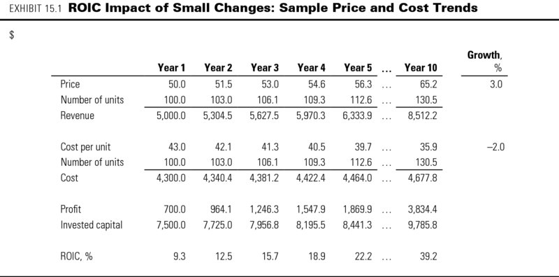
Are the patterns consistent with industry dynamics? In certain cases, reasonable changes in key inputs can lead to unintended consequences. Exhibit 15.1 presents price and cost data for a hypothetical company in a competitive industry. To keep pace with inflation, you forecast the company's prices to increase by 3 percent per year. Because of cost efficiencies, operating costs are expected to drop by 2 percent per year. In isolation, each rate appears innocuous. Computing ROIC reveals a significant trend. Between year 1 and year 10, ROIC grows from 9.3 to 39.2 percent—unlikely in a competitive industry. Since cost advantages are difficult to protect, competitors are likely to mimic production and lower prices to capture share. A good model will highlight this economic inconsistency.
Is the company in a steady state by the end of the explicit forecasting period? Following the explicit forecasting period, when you apply a continuing-value formula, the company's margins, returns on invested capital, and growth should be stable. If this is not the case, extend the explicit forecast period until a steady state is reached.

Are the Results Plausible?

Once you believe the model is technically sound and economically consistent, you should test whether its valuation results are plausible. If the company is listed, compare your results with the market value. If your estimate is far from the market value, do not jump to the conclusion that the market is wrong. Your default assumption should be that the market is right, unless you have specific indications that not all relevant information has been incorporated in the share price—for example, due to a small free float or low liquidity of the stock.

Also perform a sound multiples analysis. Calculate the implied forward-looking valuation multiples of the operating value over, for example, earnings before interest, taxes, and amortization (EBITA). Compare these with equivalently defined multiples of traded peer-group companies. Chapter 16 describes how to do a proper multiples analysis. Make sure you can explain any significant differences with peer-group companies in terms of the companies' value drivers and underlying business characteristics or strategies.

Sensitivity Analysis

With a robust model in hand, test how the company's value responds to changes in key inputs. Senior management can use sensitivity analysis to prioritize the actions most likely to affect value materially. From the investor's perspective, sensitivity analysis can focus on which inputs to investigate further and monitor more closely. Sensitivity analysis also helps bound the valuation range when there is uncertainty about the inputs.

Assessing the Impact of Individual Drivers

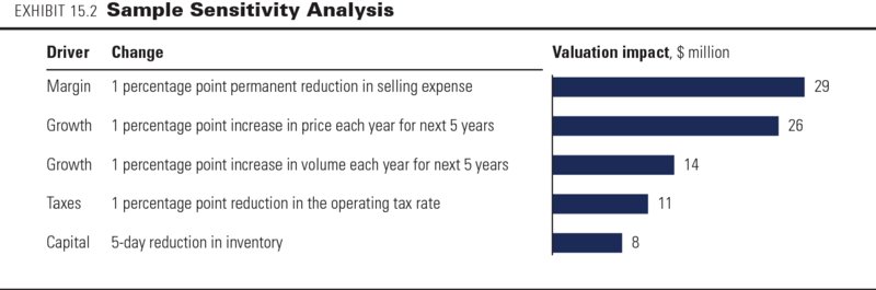
Start by testing each input one at a time to see which has the largest impact on the company's valuation. Exhibit 15.2 presents a sample sensitivity analysis. Among the alternatives presented, a permanent one-percentage-point reduction in selling expenses has the greatest effect on the company's valuation.¹ The analysis will also show which drivers have the least impact on value. Too often, we find our clients focusing on actions that are easy to measure but fail to affect value very much.

Although an input-by-input sensitivity analysis will increase your knowledge about which inputs drive the valuation, its use is limited. First, inputs rarely change in isolation. For instance, an increase in selling expenses is likely to accompany an increase in revenue growth. Second, when two inputs are changed simultaneously, interactions can cause the combined effect to differ from the sum of the individual effects. Therefore, you cannot compare a one-percentage-point increase in selling expenses with a one-percentage-point increase in growth. If there are interactions in the movements of inputs, the one-by-one analysis would miss them. To capture possible interactions, you need to analyze trade-offs.

Analyzing Trade-Offs

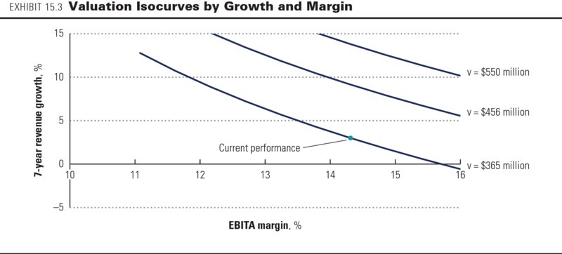
Strategic choices typically involve trade-offs between inputs into your valuation model. For instance, raising prices leads to fewer purchases, lowering inventory results in more missed sales, and entering new markets often affects both growth and margin. Exhibit 15.3 presents an analysis that measures the impact on a valuation when two inputs are changed simultaneously. Based on an EBITA margin of 14 percent and revenue growth of 3 percent (among other forecasts), a hypothetical company is currently valued at $365 million. The curve drawn through this point represents all the possible combinations of EBITA margin and revenue growth that lead to the same valuation. (Economists call this an isocurve.) To increase the valuation by 25 percent, from $365 million to $456 million, the organization needs to move northeast to the next isocurve. Using this information, management can set performance targets that are consistent with the company's valuation aspirations and competitive environment.

When performing sensitivity analysis, do not limit yourself to changes in financial variables. Check how changes in sector-specific nonfinancial value drivers affect the final valuation. This is where the model's real power lies. For example, if you increase customer churn rates for a telecommunications company, does company value decrease? Can you explain with back-of-the-envelope estimates why the change is so large or small?

Creating Scenarios

Valuation requires a forecast, but the future can take many paths. A government might pass legislation affecting the entire industry. A new discovery could revolutionize a competitor's product portfolio. Since the future is never truly knowable, consider making financial projections under multiple scenarios.2 The scenarios should reflect different assumptions regarding future macroeconomic, industry, or business developments, as well as the corresponding strategic responses by industry players. Collectively, the scenarios should capture the future states of the world that would have the most impact on value creation over time and a reasonable chance of occurrence. Assess how likely it is that the key assumptions underlying each scenario will change, and assign to each scenario a probability of occurrence.

When analyzing the scenarios, critically review your assumptions concerning the following variables:

Broad economic conditions: How critical are these forecasts to the results? Some industries are more dependent on basic economic conditions than others are. Home building, for example, is highly correlated with the overall health of the economy. Branded food processing, in contrast, is less so.
Competitive structure of the industry: A scenario that assumes substantial increases in market share is less likely in a highly competitive and concentrated market than in an industry with fragmented and inefficient competition.
Internal capabilities of the company: Focus on capabilities that are necessary to achieve the business results predicted in the scenario. Can the company develop its products on time and manufacture them within the expected range of costs?
Financing capabilities of the company: Financing capabilities are often implicit in the valuation. If debt or excess marketable securities are excessive relative to the company's targets, how will the company resolve the imbalance? Should the company raise equity if too much debt is projected? Should the company be willing to raise equity at its current market price?

Complete the alternative scenarios suggested by the preceding analyses. The process of examining initial results may well uncover unanticipated questions that are best resolved by creating additional scenarios. In this way, the valuation process is inherently circular. Performing a valuation often provides insights that lead to additional scenarios and analyses.

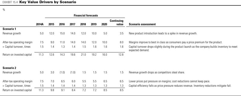
Exhibits 15.4 and 15.5 provide a simplified example of a scenario approach to discounted-cash-flow (DCF) valuation. The company being valued faces great uncertainty because of a new-product launch for which it has spent considerable time and money on research and development (think of a cosmetics company launching a new electric skin care brush, such as Pacific Bioscience's Clarisonic³). If the new product is a top seller, revenue growth will more than double over the next few years. Returns on invested capital will peak at above 20 percent and remain above 12 percent in perpetuity. If the product launch fails, however, growth will continue to erode as the company's current products become obsolete. Lower average selling prices will cause operating margins to fall. The company's returns on invested capital will decline to levels below the cost of capital, and the company will struggle to earn its cost of capital in the long term. Exhibit 15.4 presents forecasts on growth, operating margin, and capital efficiency that are consistent with each of these two scenarios.

Next, build a separate free cash flow model for each set of forecasts. Although not presented here, the resulting cash flow models are based on the DCF methodology outlined in Chapter 8. Exhibit 15.5 presents the valuation results. In the case of a successful product launch, the DCF value of operations equals $5,044 million. The nonoperating assets consist primarily of nonconsolidated subsidiaries, and given their own reliance on the product launch, they are valued at the implied NOPLAT multiple for the parent company, $672 million. A comprehensive scenario will examine all items, including nonoperating items, to make sure they are consistent with the scenario's underlying premise. Next, deduct the face value of the debt outstanding at $2,800 million (assuming interest rates have not changed, so the market value of debt equals the face value). The resulting equity value is $2,916 million.

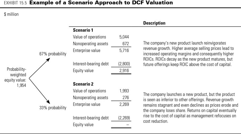
If the product launch fails, the DCF value of operations is only $1,993 million. In this scenario, the value of the subsidiaries is much lower ($276 million), as their business outlook has deteriorated due to the failure of the new product. The value of the debt is no longer $2,800 million in this scenario. Instead, the debt holders would end up with $2,269 million by seizing the enterprise. In scenario 2, the common equity would have no value.

Given the approximately two-thirds probability of success for the product, the probability-weighted equity value across both scenarios amounts to $1,954 million. Since estimates of scenario probabilities are likely to be rough at best, determine the range of probabilities that point to a particular strategic action. For instance, if this company were an acquisition target available for $1.5 billion, any probability of a successful launch above 50 percent would lead to value creation. Whether the probability is 67 percent or 72 percent does not affect the decision outcome.

When using the scenario approach, make sure to generate a complete valuation buildup from value of operations to equity value. Do not shortcut the process by deducting the face value of debt from the scenario-weighted value of operations. Doing this would seriously underestimate the equity value, because the value of debt is different in each scenario. In this case, the equity value would be undervalued by $175 million ($2,800 million face value minus $2,625 million probability-weighted value of debt).⁴ A similar argument holds for nonoperating assets.

Creating scenarios also helps you understand the company's key priorities. In our example, reducing costs or cutting capital expenditures in the downside scenario will not meaningfully affect value. Any improvements in the downside scenario whose value is less than $531 million ($2,800 million in face value less $2,269 million in market value) will accrue primarily to the debt holders. In contrast, increasing the odds of a successful launch has a much greater impact on shareholder value. Increasing the success probability from two-thirds to three-fourths would boost shareholder value by more than 10 percent.

The Art of Valuation

Valuation can be highly sensitive to small changes in assumptions about the future. Take a look at the sensitivity of a typical company with a forward-looking price-to-earnings ratio of 15 to 16. Increasing the cost of capital for this company by half a percentage point will decrease the value by approximately 10 percent. Changing the growth rate for the next 15 years by one percentage point annually will change the value by about 6 percent. For high-growth companies, the sensitivity is even greater. In light of this sensitivity, it shouldn't be surprising that the market value of a company fluctuates over time. Historical volatilities for a typical stock over the past several years have been around 25 percent per annum. Taking this as an estimate for future volatility, the market value of a typical company could well fluctuate around its expected value by 15 percent over the next month.5

We typically aim for a valuation range of plus or minus 15 percent, which is similar to the range used by many investment bankers. Even valuation professionals cannot always generate exact estimates. In other words, keep your aspirations for precision in check.

Review Questions

You are valuing DistressCo, a company struggling to hold market share. The company currently generates $120 million in revenue but is expected to shrink to $100 million next year. Cost of sales currently equals $90 million, and depreciation equals $18 million. Working capital equals $36 million, and equipment equals $120 million. Using these data, construct operating-profit and invested-capital figures for the current year. You decide to build an as-is valuation of DistressCo. To do this, you forecast each ratio (such as cost of sales to revenues) at its current level. Based on this forecast method, what are operating profits and invested capital expected to be next year? What are two critical operating assumptions (identify one for profits and one for capital) embedded in this forecast method?

You decide to value a steady-state company using probability-weighted scenario analysis. In scenario 1, NOPLAT is expected to grow at 6 percent, and ROIC equals 16 percent. In scenario 2, NOPLAT is expected to grow at 2 percent, and ROIC equals 8 percent. Next year's NOPLAT is expected to equal $100 million, and the weighted average cost of capital is 10 percent. Using the key value driver formula introduced in Chapter 2, what is the enterprise value in each scenario? If each scenario is equally likely, what is the enterprise value for the company?

A colleague recommends a shortcut to value the company in Question 2. Rather than compute each scenario separately, the colleague recommends averaging each input, such that growth equals 4 percent and ROIC equals 12 percent. Will this lead to the same enterprise value as you found in Question 2? Which method is correct? Why?

Consumer Products Co reports growth by segment in the “Management's Discussion and Analysis” section of its annual report (shown here in Exhibit 15.6, Part A) for a given year. For this year, does each segment have the same organic growth characteristics? As an approximation, set organic growth equal to the sum of volume excluding acquisitions, price, and other. Based on growth by segment, can Consumer Products Co be valued as a whole, or should individual segments be valued separately?
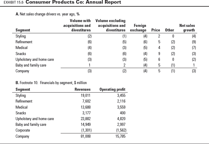
Refer to Exhibit 15.6, Part B from Consumer Products Co's annual report. Here you will find financials by segment. What are the operating margins by segment? Based on operating margin by segment, can Consumer Products Co be valued as a whole, or should individual segments be valued separately?