34
Banks

Banks are among the most complex businesses to value, especially from the outside in. Published accounts give an overview of a bank's performance, but the clarity of the picture they present depends largely on accounting decisions made by management. External analysts must therefore make a judgment about the appropriateness of those decisions. Even if that judgment is favorable, analysts are still bound to lack vital information about the bank's economics, such as the extent of its credit losses or any mismatch between its assets and liabilities, forcing them to fall back on rough estimates for their valuation. Moreover, banks are highly levered, making bank valuations even more contingent on changing economic circumstances than valuations in other sectors. Finally, most banks are in fact multibusiness companies, requiring separate analysis and valuation of their key business segments. So-called universal banks today engage in a wide range of businesses, including retail and wholesale banking, investment banking, and asset management.

In the view of some academics, managers, and regulators, the size, complexity, and lack of transparency of universal banks in the United States and Europe has led to undesirable systemic risks, among them that some banks have become “too big to fail.”1 During the 2008 credit crisis, the threat of collapse by some large universal banks led governments to bail out these institutions, triggering an ongoing debate about whether such institutions should be split into smaller and separate investment and commercial banks.²

This chapter provides a general overview of how to value banks, and highlights some of the most common valuation challenges peculiar to the sector. First it discusses the economic fundamentals of banking and trends in performance and growth, and then describes how to use the equity cash flow approach for valuing banks, using a hypothetical, simplified example. It concludes by offering some practical recommendations for valuing universal banks in all their real-world complexity.

Economics of Banking

After years of strong profitability and growth in the U.S. and European banking sectors, the crisis in the mortgage-backed securities market in 2007 sent many large banks spiraling into financial distress. Many large institutions on either side of the Atlantic went bankrupt or were kept afloat with costly government bailouts. The fallout in the real economy from what was originally a crisis in the banking sector ultimately curtailed growth in almost all sectors around the globe, bringing economic growth to a halt worldwide in 2008.

Since then, the sector has gone through years of restructuring, involving mergers, government bailouts, nationalizations, and bankruptcies. Regulation has intensified, leading to stricter capital requirements, restrictions on trading operations, and—in some European countries—caps on bonus payments for bank employees and executives. By 2014, banks in the United States had ridden stronger domestic economic growth, rebounding loan demand, and a reduction in bad debts to regain their pre-crisis profit levels. In contrast, European banks were still far below their pre-crisis profit levels due to a lack of economic growth across the European Union and the 2010 euro sovereign-debt crisis.

The credit crisis demonstrates the extent to which the banking industry is both a critical and a vulnerable component of modern economies. Banks are vulnerable because they are highly leveraged and their funding depends on investor and customer confidence. This can disappear overnight, sending a bank plummeting into failure. As a result, more uncertainty surrounds the valuation of banks than the valuation of most industrial companies. Therefore, it is all the more important for anyone valuing a bank to understand the business activities undertaken by banks, the ways in which banks create value, and the drivers of that value creation.

Universal banks may engage in any or all of a wide variety of business activities, including lending and borrowing, underwriting and placement of securities, payment services, asset management, proprietary trading, and brokerage. For the purpose of financial analysis and valuation, we group these activities according to the three types of income they generate for a bank: net interest income, fee and commission income, and trading income. “Other income” forms a fourth and generally smaller residual category of income from activities unrelated to the main banking businesses.

Net Interest Income

In their traditional role, banks act as intermediaries between parties with funding surpluses and those with deficits. They attract funds in the form of customer deposits and debt to provide funds to customers in the form of loans such as mortgages, credit card loans, and corporate loans. The difference between the interest income a bank earns from lending and the interest expense it pays to borrow funds is its net interest income. For the regional retail banks in the United States and retail-focused universal banks such as Standard Chartered, Banco Santander, and Unicredit, net interest income typically forms around half of total net revenues.

As discussed later in this chapter, it is important to understand that not all of a bank's net interest income creates value. Most banks have a maturity mismatch as a result of using short-term deposits as funding to back long-term loans and mortgages. In this case, the bank earns income from being on different parts of the yield curve. Typically, borrowing for the short term costs less than what the bank can earn from long-term lending. Yet it is unclear whether all of this income represents value creation. For example, the true value created from lending is measured by the difference between the rate that banks receive on their outstanding loans and their returns in the financial markets on loans with the same maturity (see the section on economic-spread analysis later in this chapter).

Fee and Commission Income

For services such as transaction advisory, underwriting and placement of securities, managing investment assets, securities brokerage, and many others, banks typically charge their customers a fee or commission. For investment banks (such as Morgan Stanley) and for universal banks with large investment banking activities (among them HSBC, Bank of America, and Deutsche Bank), commission and fee income makes up around half of total net revenues. Fee income is usually easier to understand than net interest income, as it is independent of financing. However, some forms of fee income are highly cyclical; examples include fees from underwriting and transaction advisory services.

Trading Income

Over the past 30 years, proprietary trading emerged as a third main category of income for the banking sector as a whole. This can involve not only a wide variety of instruments traded on exchanges and over the counter, such as equity stocks, bonds, and foreign exchange, but also more exotic products, such as credit default swaps and asset-backed debt obligations, traded mostly over the counter.

Trading profits tend to be highly volatile: gains made over several years may be wiped out by large losses in a single year, as the credit crisis painfully illustrated. These activities have also attracted considerable attention in the wake of the crisis. In 2010, the United States adopted legislation preventing banks from engaging in proprietary trading for their own profit.3 This resulted in steeply lower overall trading income, as the law permits only trading related to serving the bank's customers. Similar restrictions were adopted in Europe, and though they have not yet been enforced there, trading income for European banks has sharply declined since 2008.

Other Income

Some banks also generate income from a range of nonbanking activities, including real estate development, minority investments in industrial companies, and distribution of investment, insurance, and pension products and services for third parties. Typically, these activities make only small contributions to overall income and are unrelated to the bank's main banking activities.

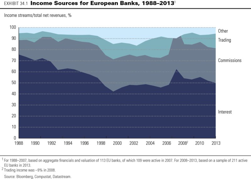
As Exhibit 34.1 shows for the European banking sector, the relative importance of these four income sources has changed radically over past decades. European banks have steadily shifted away from interest income toward commission and trading income. However, trading income collapsed during the credit crisis. Despite recovering somewhat since then, in 2014 it was still running far below its pre-crisis levels.

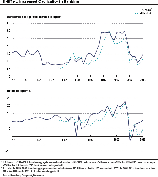
As the banks have shifted their sources of income, the cyclicality of their profitability and market valuations has increased. This is measured by their return on equity and their market-to-book ratios (see Exhibit 34.2). The return on equity and market-to-book ratios for the sector as a whole in both the United States and Europe rose sharply after 1995 to reach historic peaks in 2006. But they fell sharply during the credit crisis, with European banks suffering a second decline during the 2010 euro bond crisis. In 2014, profitability and valuation levels remained far below their peak levels on both sides of the Atlantic, though American banks were much more successful than their European counterparts in regaining some ground.

Principles of Bank Valuation

Throughout most of this book, we apply the enterprise discounted-cash-flow (DCF) approach to valuation. Discounting free cash flows is the appropriate approach for nonfinancial companies where operating decisions and financing decisions are separate. For banks, however, we cannot value operations separately from interest income and expense, since these are the main categories of a bank's core operations. It is necessary to value the cash flow to equity, which includes both the operational and financial cash flows. For valuation of banks, we therefore recommend the equity DCF method.4 To understand the principles of the equity DCF method, let's explore a stylized example of a retail bank. ABC Bank attracts customer deposits to provide funds for loans and mortgages to other customers. ABC's historical balance sheet, income statement, and key financial indicators are shown in Exhibit 34.3.

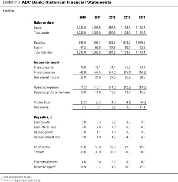
At of the start of 2014, the bank has $1,134 million of loans outstanding with customers, generating 6.5 percent interest income. To meet regulatory requirements, ABC must maintain an 8 percent ratio of Tier 1 equity capital to loan assets, which we define for this example as the ratio of equity divided by total assets. This means that 8 percent, or $91 million, of its loans are funded by equity capital, and the rest of the loans are funded by $1,043 million of deposits. The deposits carry 4.3 percent interest, generating total interest expenses of $45 million.

Net interest income for ABC amounted to $29 million in 2014, thanks to the higher rates received on loans than paid on deposits. All capital gains or losses on loans and deposits are included in interest income and expenses. Operating expenses such as labor and rental costs are $13 million, which brings ABC's cost-to-income ratio to 45 percent of net interest income. After subtracting taxes at 30 percent, net income equals $11 million, which translates into a return on equity of 12.2 percent.

As discussed in Chapter 8, the equity value of a company equals the present value of its future cash flow to equity (CFE), discounted at the cost of equity, k_e:

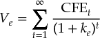
We can derive equity cash flow from two starting points. First, equity cash flow equals net income minus the earnings retained in the business:

where CFE is equity cash flow, NI is net income, ΔE is the increase in the book value of equity, and OCI is noncash other comprehensive income.

Net income represents the earnings theoretically available to shareholders after payment of all expenses, including those to depositors and debt holders. However, net income by itself is not cash flow. As a bank grows, it will need to increase its equity; otherwise, its ratio of debt plus deposits over equity would rise, which might cause regulators and customers to worry about the bank's solvency. Increases in equity reduce equity cash flow, because they mean the bank is issuing more shares or setting aside earnings that could otherwise be paid out to shareholders. The last step in calculating equity cash flow is to add noncash other comprehensive income, such as net unrealized gains and losses on certain equity and debt investments, hedging activities, adjustments to the minimum pension liability, and foreign-currency translation items. This cancels out any noncash adjustment to equity.⁵

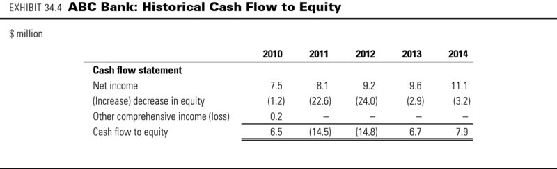
Exhibit 34.4 shows the equity cash flow calculation for ABC Bank. Note that in 2010, ABC's other comprehensive income includes a translation gain on its overseas loan business, which was discontinued in the same year. ABC's cash flow to equity was negative in 2011 and 2012 because it raised new equity to lift its Tier 1 ratio from 4 percent to 8 percent.

Another way to calculate equity cash flow is to sum all cash paid to or received from shareholders, including cash changing hands as dividends, through share repurchases, and through new share issuances. Both calculations arrive at the same result. Note that equity cash flow is not the same as dividends paid out to shareholders, because share buybacks and issuance can also form a significant part of cash flow to and from equity.

Analyzing and Forecasting Equity Cash Flows

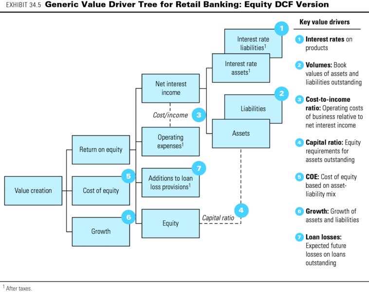
The generic value driver tree for a retail bank, shown in Exhibit 34.5, is conceptually the same as one for an industrial company. Following the tree's branches, we analyze ABC's historical performance as laid out in Exhibit 34.3.

Over the past five years, ABC's loan portfolio has grown by around 3.0 to 3.5 percent annually. Since 2010, ABC's interest rates on loans have been declining from 7.0 percent to 6.5 percent in 2014, but this was offset by an even stronger decrease in rates on deposits from 5.0 percent to 4.3 percent over the same period. Combined with the growth in its loan portfolio, this lifted ABC's net interest income from $22 million in 2010 to $29 million in 2014. The bank also managed to improve its cost-to-income ratio significantly from a peak level of 53 percent in 2011 to 45 percent in 2014.

Higher regulatory requirements for equity risk capital forced ABC to double its Tier 1 ratio (equity to total assets) from 4 percent to 8 percent over the period. The combination of loan portfolio growth and stricter regulatory requirements has forced ABC to increase its equity capital by some $50 million since 2009. As a result, ABC's return on equity declined significantly in 2014 to 12 percent, from nearly 20 percent in 2011.

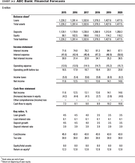
Exhibit 34.6 shows the financial forecasts for ABC Bank, assuming its loan portfolio growth rate increases to 4.5 percent in the short term and settles at 3.5 percent in perpetuity. Interest rates on loans and deposits are expected to decrease to 6.1 and 3.9 percent, respectively. Operating expenses will decline to 43 percent of net interest income. As a result, ABC's return on equity increases somewhat to 12.8 percent in 2016 and stays at that level in perpetuity. Note that a mere one-percentage-point increase in interest rates on loans would translate into a change in return on equity of around 12 percentage points, a function of ABC's high leverage (equity capital at 8 percent of total assets).

Discounting Equity Cash Flows

To estimate the cost of equity, k_e, for ABC Bank, we use a beta of 1.3 (based on the average beta for its retail banking peers), a long-term risk-free interest rate of 4.5 percent, and a market risk premium of 5 percent:6

where r_f is the risk-free rate, β is the equity beta, and MRP is the market risk premium. (Because we discount at the cost of equity, there is no need to adjust any estimates of equity betas of banking peers for leverage when deriving ABC's equity beta.)

In the equity DCF approach, we use an adapted version of the value driver formula presented in Chapter 2, replacing return on invested capital (ROIC) and return on new invested capital (RONIC) with return on equity (ROE) and return on new equity investments (RONE), and replacing net operating profit less adjusted taxes (NOPLAT) with net income:

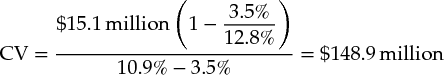
where CV_t is the continuing value as of year t, NI_t+1 is the net income in year t + 1, g equals growth, and k_e is the cost of equity.

Assuming that ABC Bank continues to generate a 12.8 percent ROE on its new business investments in perpetuity while growing at 3.5 percent per year,⁷ its continuing value as of 2020 is as follows:

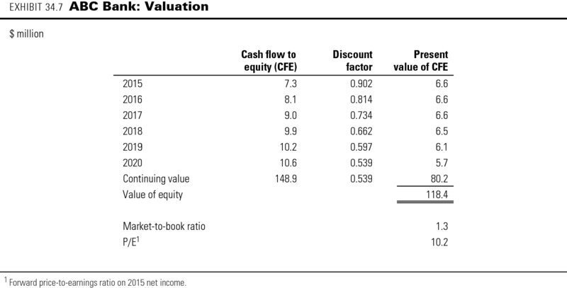
The calculation of the discounted value of ABC's cash flow to equity is presented in Exhibit 34.7. The present value of ABC's equity amounts to $118 million, which implies a market-to-book ratio for its equity of 1.3 and a price-to-earnings (P/E) ratio of 10.2. As for industrial companies, whenever possible you should triangulate your results with an analysis based on multiples (see Chapter 16). Note that the market-to-book ratio indicates that ABC is creating value over its book value of equity, which is consistent with a long-term return on equity of 12.8 percent (which is above the cost of equity of 10.9 percent).

Pitfalls of Equity DCF Valuation

The equity DCF approach as illustrated here is straightforward and theoretically correct. However, the approach involves some potential pitfalls. These concern the sources of value creation, the impact of leverage and business risk on the cost of equity, and the tax penalty on holding equity risk capital.

Sources of value creation

The equity DCF approach does not tell us how and where ABC Bank creates value in its operations. Is ABC creating or destroying value when receiving 6.5 percent interest on its loans or when paying 4.3 percent on deposits? To what extent does ABC's net income reflect intrinsic value creation?

You can overcome this pitfall by undertaking economic-spread analysis, described in the next section. As that section will show, ABC is creating value in its lending business but much less so in deposits, which were not creating any value before 2014 in this particular example. A significant part of ABC's net interest income in 2014 is, in fact, driven by the mismatch in maturities of its short-term borrowing and long-term lending. The mismatch in itself does not necessarily create any value for shareholders, because they could set up a similar position in the bond market. The key question is whether ABC Bank can attract deposits and provide loans at better-than-market interest rates—and this is addressed by economic-spread analysis.

Impact of leverage and business risk on cost of equity

As for industrial companies, the cost of equity for a bank such as ABC should reflect its business risk and leverage. Its equity beta is a weighted average of the betas of all its loan and deposit businesses. So when you project significant changes in a bank's asset or liability composition or equity capital ratios, you cannot leave the cost of equity unchanged.

For instance, if ABC were to decrease its equity capital ratio, its expected return on equity would go up. But in the absence of taxes, by itself this should not increase the intrinsic equity value, because ABC's cost of equity would also rise, as its cash flows would now be more risky. It will increase ABC's value only to the extent that the bank is creating value on the deposit business that it is growing as a result of the leverage increase (see next section, on economic-spread analysis).8

The same line of reasoning holds for changes in the asset or liability mix. Assume ABC raises an additional $50 million in equity and invests this in government bonds at the risk-free rate of 4.5 percent, reducing future returns on equity. If you left ABC's cost of equity unchanged at 10.9 percent, the estimated equity value per share would decline. But in the absence of taxation, the risk-free investment cannot be value-destroying, because its expected return exactly equals the cost of capital for risk-free assets. There is no impact on value creation if we assume that the bank has no competitive (dis)advantage in investing in government bonds. The assumption seems reasonable, as it implies that the bank does not obtain the government bonds at a premium or discount to their fair market value. As a result, if you accounted properly for the impact of the change in its asset mix on the cost of equity and the resulting reduction in the beta of its business, ABC's equity value would remain unchanged.

Tax penalty on holding equity risk capital

Holding equity risk capital represents a cost for banks, and it is important to understand what drives this cost. Consider again the example of ABC Bank issuing new equity and investing in risk-free assets, thereby increasing its equity risk capital. In the absence of taxation, this extra layer of risk capital would have no impact on value, and there would be no cost to holding it. But interest income is taxed, and that is what makes holding equity risk capital costly; equity, unlike debt or deposits, provides no tax shield. In this example, ABC will pay taxes on the risk-free interest income from the $50 million of risk-free bonds that cannot be offset by tax shields on interest charges on deposits or debt, because the investment was funded with equity, for which there are no tax-deductible interest charges.

The true cost of holding equity capital is this so-called tax penalty, whose present value equals the equity capital times the tax rate. If ABC Bank were to increase its equity capital by $50 million to invest in risk-free bonds, holding everything else constant, this would entail destroying $15 million of present value (30 percent times $50 million) because of the tax penalty. As long as the cost of equity reflects the bank's leverage and business risk, the tax penalty is implicitly included in the equity DCF. However, in the economic-spread analysis discussed next, we explicitly include the tax penalty as a cost of the bank's lending business.

Economic-Spread Analysis

Because the equity DCF approach does not reveal the sources of value creation in a bank, some further analysis is required. To understand how much value ABC Bank is creating in its different product lines, we can analyze them by their economic spread.9 We define the pretax economic spread on ABC's loan business in 2014 as the interest rate on loans minus the matched-opportunity rate (MOR) for loans, multiplied by the amount of loans outstanding at the beginning of the year:

where S_BT is the pretax spread, L is the amount of the loans, r_L is the interest rate on the loans, and k_L is the MOR for the loans.

The matched-opportunity rate is the cost of capital for the loans—that is, the return the bank could have captured for investments in the financial market with similar duration and risk as the loans. Note that the actual interest rate a bank is paying for deposit or debt funding is not necessarily relevant, because the maturity and risk of its loans and mortgages often do not match those of its deposits and debt. For example, the MOR for high-quality four-year loans should be close to the yield on investment-grade corporate bonds with four years to maturity that are traded in the market. Banks create value on their loan business if the loan interest rate is above the matched-opportunity rate.

To obtain the economic spread after taxes (S_AT), it is necessary to deduct the taxes on the spread itself, a tax penalty on the equity required for the loan business (TPE), and the tax on any maturity mismatch in the funding of the loans (TMM):

The tax penalty on equity occurs because, in contrast to deposit and debt funding, equity provides no tax shield, as dividend payments are not tax deductible.¹⁰ Thus, the more a bank relies on equity funding instead of deposits or debt, the less value it creates, everything else being equal. Of course, banks have to fund their operations at least partly with equity. One reason is that regulators in most countries have established solvency restrictions that require banks to hold on to certain minimum equity levels relative to their asset bases. In addition, banks with little or no equity funding would not be able to attract deposits from customers or debt, because their default risk would be too high. For ABC's loan business, this tax penalty in 2014 is calculated as follows:¹¹

where e_L is the required equity capital divided by the amount of loans outstanding and k_D is the MOR for deposits.

In addition, the tax on a maturity mismatch (TMM) needs to be included if the maturity of the loans does not correspond to that of the bank's deposits. Typically, the maturity of a bank's loans is longer than that of the deposits by which it funds its operations, and a difference arises in the matched-opportunity rates. For example, in the case of ABC Bank, the loans have a longer maturity than the deposits. As a result, the MOR for loans (5.1 percent) is above the MOR for deposits (4.6 percent). The maturity difference in itself does not create or destroy any value, as it does not affect the economic spread on deposits or loans. But the taxation of the interest income that the mismatch generates has an impact on value, which should be included in the economic spread on loans. Note that the tax result on the maturity mismatch could be positive in the (unlikely) case that a bank's loans have a shorter maturity than its deposits. The TMM for ABC Bank's loans in 2014 is calculated as follows:

The after-tax economic spread on loans is then derived as:

This number represents the dollar amount of value created by ABC's loan business. Along the same lines, we can define the economic spread for ABC Bank's deposit products as well (see Exhibit 34.8). Our analysis explicitly includes the spread on deposits because banks (in contrast to industrial companies) aim to create value in their funding operations. For example, ABC Bank created value for its shareholders in its deposit business in 2014 because it attracted deposits at a 4.3 percent interest rate, below the 4.6 percent rate for traded bonds with the same high credit rating as ABC had.¹²

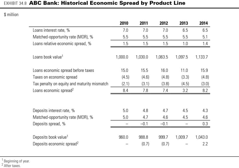
When comparing the spread across ABC product lines over the past few years, we can immediately see that most of the value created comes from its lending business. In fact, ABC was not making any money on its deposit funding from 2009 to 2013, as shown by the zero or negative spreads in those years.

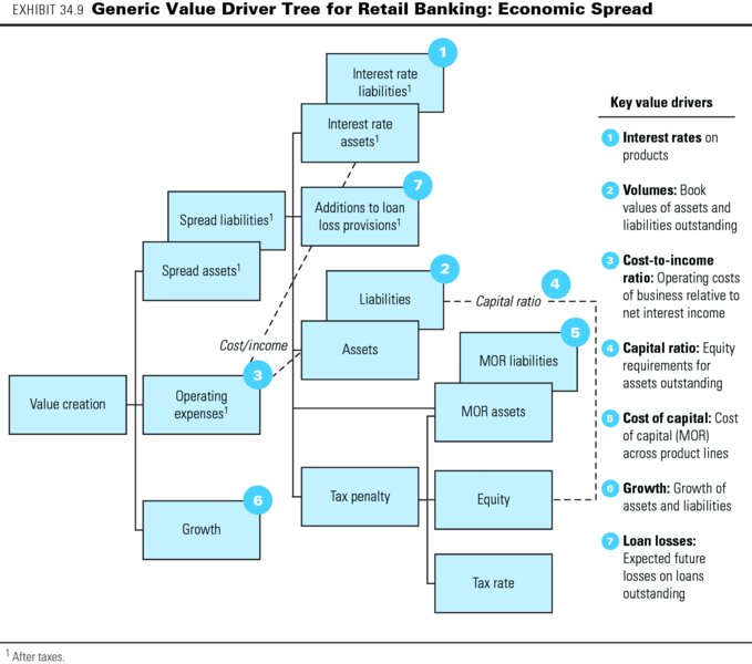
From our calculations of the economic spreads of the two businesses, it is possible to rearrange the value driver tree from the equity DCF approach shown previously in Exhibit 34.5. In the revised value driver tree shown in Exhibit 34.9, the key drivers are virtually identical but highlight some important messages about value creation for banks:

• Interest income on assets creates value only if the interest rate exceeds the cost of capital for those assets (i.e., the matched-opportunity rate) by more than the taxes on any maturity mismatch.
• Changes in the capital ratio affect value creation only through the tax penalty on equity.
• Growth adds value only if the economic spread from the additional product sold is positive and sufficient to cover any operating expenses.

Note that we could further refine the tree by allocating the operating expenses to the product lines, represented by the different asset and liability categories. This is worth doing if there is enough information on the operating costs incurred by each product line and the equity capital required for each.

Economic Spread vs. Net Interest Income

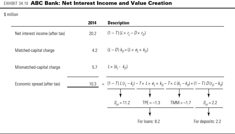
The spread analysis helps to show why a bank's reported net interest income does not reveal the value created by the bank and should be interpreted with care. For example, out of ABC Bank's 2014 net interest income after taxes of $20.2 million, only $10.3 million represents true value created (the economic spread of $8.2 million on loans plus $2.2 million on deposits minus a rounding difference, as shown in Exhibit 34.10). The remaining $9.9 million is income but not value, because it is offset by the following two charges shown in the exhibit:

1. The matched-capital charge, amounting to $4.2 million for ABC in 2014, is the income that would be required on assets and liabilities if there were no maturity mismatch and no economic spread. In that case, all assets and liabilities would have identical duration (and risk) to deposits, so that their return would equal k_D (the MOR on deposits) and net interest income would equal equity times k_D. This component of net interest income does not represent value; it only provides shareholders the required return on their equity investment in a perfectly matched bank.¹³
2. The mismatched-capital charge, amounting to $5.7 million of ABC's net interest income, arises from the difference in the duration of ABC's assets and deposits. To illustrate, when a bank borrows at short maturity and invests at long maturity, it creates income. The income does not represent value when the risks of taking positions on the yield curve are taken into account. The mismatched-capital charge represents the component of net interest income required to compensate shareholders for that risk.¹⁴

Because economic-spread analysis provides such insights into value creation across a bank's individual product lines, we recommend using it to understand a bank's performance. We recommend using the DCF model to perform the valuation of the bank.

Complications in Bank Valuations

When you value banks, significant challenges arise in addition to those discussed in the hypothetical ABC Bank example. In reality, banks have many interest-generating business lines, including credit card loans, mortgage loans, and corporate loans, all involving loans of varying maturities. On the liability side, banks could carry a variety of customer deposits as well as different forms of straight and hybrid debt. Banks need to invest in working capital and in property, plant, and equipment, although the amounts are typically small fractions of total assets. Obviously, this variety makes the analysis of real-world banks more complex, but the principles laid out in the ABC example remain generally applicable. This section discusses some practical challenges in the analysis and valuation of banks.

Convergence of Forward Interest Rates

For ABC Bank, we assumed a perpetual difference in short-term and long-term interest rates. As a result, ABC generates a permanent, positive net interest income from a maturity mismatch: using short-term customer deposits as funding for investments in long-term loans. However, following the expectations theory of interest rates, long-term rates move higher when short-term rates are expected to increase, and vice versa. Following this theory, it is necessary to ensure that our expectations for interest rates in future years are consistent with the current yield curve.

Exhibit 34.11 shows an example of a set of future one-, three-, five-, and ten-year interest rates that are consistent with the yield curve as of 2014. The forecasts for a bank's interest income and expenses should be based on these forward rates, which constitute the matched-opportunity rates for the different product lines. For example, if the bank's deposits have a three-year maturity on average, you should use the interest rates from the forward three-year interest rate curve minus an expected spread for the bank to forecast the expected interest rates on deposits in your DCF model. The rates are all derived from the current yield curve. To illustrate, the expected three-year interest rate in 2016 follows from the current three- and six-year yield:

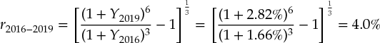
where r_2016–2019 is the expected three-year interest rate as of 2016, Y₂₀₁₆ is the current three-year interest rate, and Y₂₀₁₉ is the current six-year interest rate.

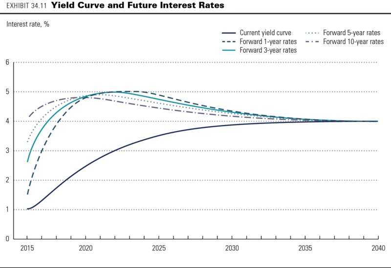
In practice, forward rate curves derived from the yield curve will rarely follow the smooth patterns of Exhibit 34.11. Small irregularities in the current yield curve can lead to large spikes and dents in the forward rate curves, which would produce large fluctuations in net interest income forecasts. As a practical solution, use the following procedure. First, obtain the forward one-year interest rates from the current yield curve. Then smooth these forward one-year rates to even out the spikes and dents arising from irregularities in the yield curve. Finally, derive the two-year and longer-maturity forward rates from the smoothed forward one-year interest rates. As the exhibit shows, all interest rates should converge toward the current yield curve in the long term. As a result, the bank's income contribution from any maturity difference in deposits and loans disappears in the long term as well.

Loan Loss Provisions

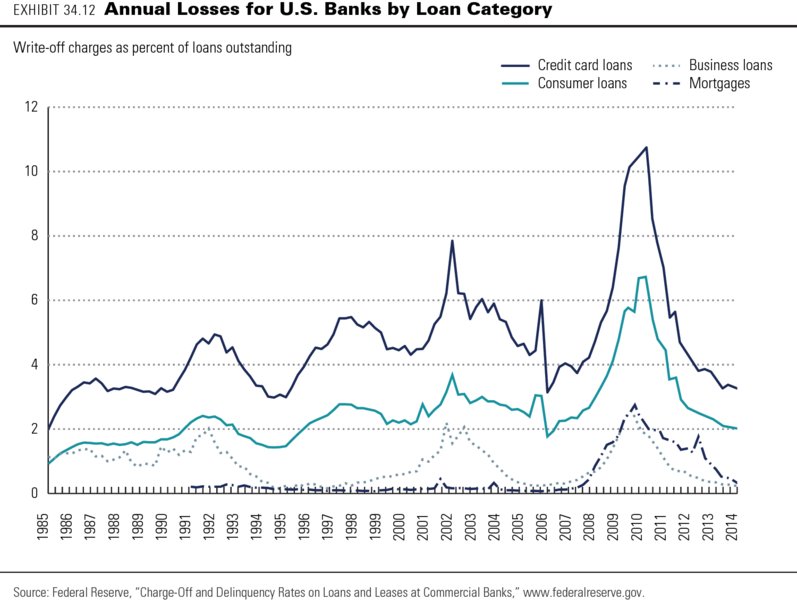
For our ABC Bank valuation, we did not model any losses from defaults on loans outstanding to customers. In real life, your analysis and valuation have to include loan loss forecasts, because loan losses are among the most important factors determining the value of retail and wholesale banking activities. For estimating expected loan losses from defaults across different loan categories, a useful first indicator would be a bank's historical additions to loan loss provisions or sector-wide estimates of loan losses (see Exhibit 34.12). As the exhibit shows, these losses increased sharply during the 2008 credit crisis but recovered to pre-crisis levels by 2013. Credit cards typically have the highest losses, and mortgages the lowest, with business loans somewhere in between. All default losses are strongly correlated with overall economic growth, so use through-the-economic-cycle estimates of additions to arrive at future annual loan loss rates to apply to your forecasts of equity cash flows.

To project the future interest income from a bank's loans, deduct the estimated future loan loss rates from the future interest rates on loans for each year. You should also review the quality of the bank's current loan portfolio to assess whether it is under- or overprovisioned for loan losses. Any required increase in the loan loss provision translates into less equity value. Many banks may need to make such an increase in the wake of the credit crisis.

Risk-Weighted Assets and Equity Risk Capital

Banks are required to hold a minimum level of equity capital that can absorb potential losses to safeguard the bank's obligations to its customers and financiers. In December 2010, new regulatory requirements for capital adequacy were specified in the Basel III guidelines, replacing the 2007 Basel II accords, which were no longer considered adequate in the wake of the 2008 and 2010 financial crises.15 The new guidelines are being gradually implemented by banks across the world between 2013 and 2019.

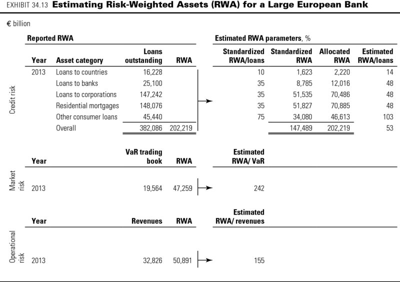
Basel III specifies rules for banks regarding how much equity capital they must hold based on the bank's so-called risk-weighted assets (RWA).¹⁶ The level of RWA is driven by the riskiness of a bank's asset portfolio and its trading book. Banks have some flexibility to choose either internal risk models or standardized Basel approaches to estimate their RWA. All such models rest on the general principle that the total RWA is the sum of separate RWA estimates for credit risk, market risk, and operational risk. However, banks do not publish the risk models they use. If you are conducting an outside-in valuation, you need an approximation of a bank's future equity risk capital needs. Because banks typically provide information on total RWA but not on the risk weighting for its asset groups, trading book, and operations, you have to make an approximation of the key categories' contribution to total RWA for the bank in order to project RWA and risk capital for future years.¹⁷

Exhibit 34.13 shows such an outside-in approximation of RWA for a large European bank. The bank separately reports the total RWA for credit risk, market risk, and operational risk.

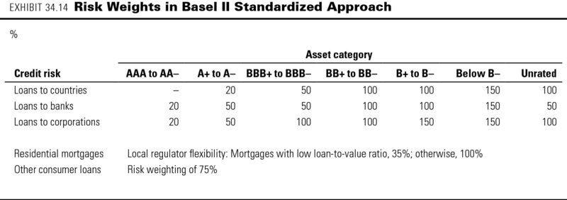
• To approximate the RWA for credit risk, you can use the risk weights from the Basel II Standardized Approach (see Exhibit 34.14) and information on the credit quality of the bank's loans. Estimate the risk weighting and RWA for each of the loan categories in such a way that your estimate fits the reported RWA for all loans (€202 billion in this example).
• Market risk is a bank's exposure to changes in interest rates, stock prices, currency rates, and commodity prices. It is typically related to its value at risk (VaR), which is the maximum loss for the bank under a worst-case scenario of a given probability for these market prices. For an approximation, use the reported VaR over several years to estimate the bank's RWA as a percentage of VaR (242 percent in the example).
• Operational risk is all risk that is neither market nor credit risk. It is usually related to a bank's net revenues (net interest income plus net other income). Use the bank's average revenues over the previous year(s) to estimate RWA per unit of revenue (155 percent in the example).

Based on your forecasts for growth across different loan categories, VaR requirements for trading activities, and a bank's net revenues, you can estimate the total RWA in each future year.

Basel III establishes stricter rules for banks regarding how much capital they must hold based on their level of RWA. Requirements are defined for the bank's so-called common-equity Tier 1 (CET1), additional Tier 1, and Tier 2 capital levels, relative to RWA. Of these capital ratios, CET1 to RWA is typically the most stringent. The total minimum CET1 requirements for a bank consist of different layers that add up to a total of 7.0 to 9.5 percent of RWA:

Basel III CET1 capital requirements
Percent of risk-weighted assets
Legal minimum	4.5
Capital conservation buffer	2.5
G-SIB countercyclical buffer	0.0–2.5
Total	7.0–9.5

The first 4.5 percent is the so-called legal minimum that applies to any bank in any given year. The second layer of 2.5 percent is the capital conservation buffer, which can be drawn down in years of losses and then rebuilt in profitable years. The third, or countercyclical, layer can be up to 2.5 percent of RWA but applies only to so-called global systemically important banks (G-SIBs). These banks are identified by the Financial Stability Board (FSB) as sources of systemic risk to the international financial system because of their size and complexity.¹⁸ In November of each year, the FSB publishes the additional capital charge for each G-SIB, which depends on the FSB's assessment of the risk that the bank represents. In 2013, some of the largest global banks, such as Citigroup, JPMorgan Chase, Deutsche Bank, and HSBC, faced a surcharge of 2.5 percent. For the next tier of G-SIBs, such as Santander, Crédit Agricole, and Wells Fargo, the surcharge amounted to 1.0 percent.

Although the new Basel capital adequacy rules are not fully phased in until 2019, many banks nowadays already target CET1 at around 10 percent of RWA, anticipating not only the new regulations but also increased investor requirements. According to the Bank for International Settlements (BIS), the worldwide average CET1 for large international banks as well as smaller regional banks was at 9.5 percent of RWA in 2013.¹⁹

Using your RWA forecasts and the targeted CET1 ratio, you can estimate the required Tier 1 capital in each future year. From the projected CET1 capital requirements, you can estimate the implied shareholders' equity requirements by applying an average historical ratio of CET1 capital to shareholders' equity excluding goodwill and deferred-tax assets. Historical Tier 1 capital is reported separately in the notes to the bank's financial statements and is typically close to straightforward shareholders' equity excluding goodwill and deferred-tax assets.

Value Drivers for Different Banking Activities

Given that many banks have portfolios of different business activities, sometimes as distinct as consumer credit card loans and proprietary trading, their businesses can have very distinct risks and returns, making the bank's consolidated financial results difficult to interpret, let alone forecast. The businesses are best valued separately, as in the case of multibusiness companies, discussed in Chapter 17. Unfortunately, financial statements for multibusiness banks often lack separately reported income statements and balance sheets for different business activities. In that case, you have to construct separate statements following the guidelines described in Chapter 17.

Interest-generating activities

Retail banking, credit card services, and wholesale lending generate interest income from large asset positions and risk capital. These interest-generating activities can be analyzed using the economic-spread approach and valued using the equity DCF model, as discussed for ABC Bank in the previous section.

Trading activities

Like a bank's interest-generating activities, its trading activities also generate income from large asset positions and significant risk capital. However, trading incomes tend to be far more volatile than interest incomes. Although peak income can be very high, the average trading income across the cycle generally turns out to be limited. The key value drivers are shown in Exhibit 34.15, a simplified value driver tree for trading activities.

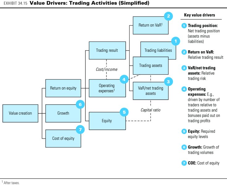
You can think of a bank's trading results as driven by the size of its trading positions, the risk taken in trading (as measured by the total VaR), and the trading result per unit of risk (measured by return on VaR). The ratio of VaR to net trading position is an indication of the relative risk taking in trading. The more risk a bank takes in trading, the higher the expected trading return should be, as well as the required risk capital. The required equity risk capital for the trading activities follows from the VaR (and RWA), as discussed earlier in the chapter. Operating expenses, which include information technology (IT) infrastructure, back-office costs, and employee compensation, are partly related to the size of positions (or number of transactions) and partly related to trading results (e.g., employee bonuses).

Fee- and commission-generating activities

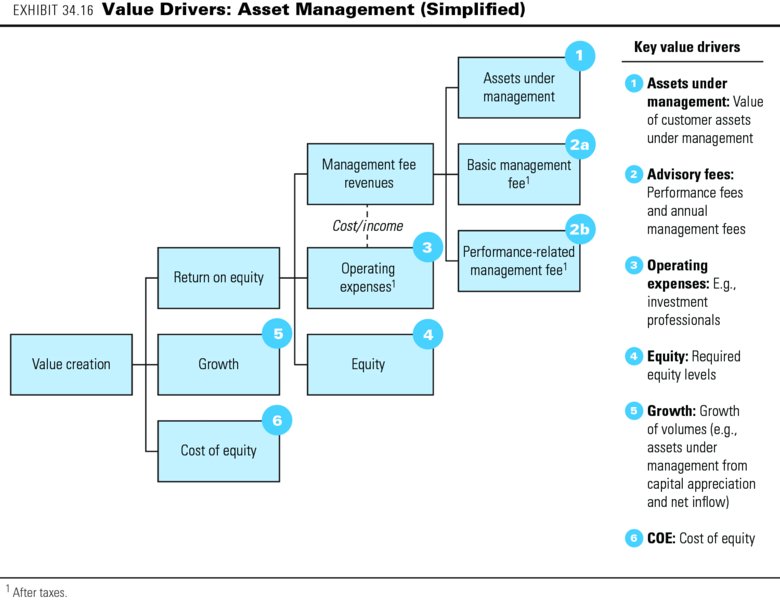
A bank's fee- and commission-generating activities, such as brokerage, transaction advisory, and asset management services, have different economics, based on limited asset positions and minimal risk capital. The value drivers in asset management, for example, are very different from those in the interest-generating businesses, as the generic example in Exhibit 34.16 shows. Key drivers are the growth of assets under management and the fees earned on those assets, such as management fees related to the amount of assets under management and performance fees related to the returns achieved on those assets.

Along with these variables in activities, remember that banks are highly leveraged and that many of their businesses are cyclical. When performing a bank valuation, you should not rely on point estimates but should use scenarios for future financial performance to understand the range of possible outcomes and the key underlying value drivers.

Summary

The fundamentals of the discounted-cash-flow (DCF) approach laid out in this book apply equally to banks. The equity cash flow version of the DCF approach is most appropriate for valuing banks, because the operational and financial cash flows of these organizations cannot be separated, given that banks are expected to create value from funding as well as lending operations.

Valuing banks remains a delicate task because of the diversity of the business portfolio, the cyclicality of many bank businesses (especially trading and fee-based business), and high leverage. Because of the difference in underlying value drivers, it is best to value a bank by its key parts according to the source of income: interest-generating business, fee and commission business, and trading. To understand the sources of value creation in a bank's interest-generating business, supplement the equity DCF approach with an economic-spread analysis. This analysis reveals which part of a bank's net interest income represents true value creation and which reflects not value but charges for maturity mismatch and capital. When forecasting a bank's financials, handle the uncertainty surrounding the bank's future performance and growth by using scenarios that capture the cyclicality of its key businesses.

Review Questions

1. Why should you estimate the value of a bank by employing the equity cash flow method, rather than the enterprise DCF models stressed throughout the text?
2. Identify the value drivers embedded in the equity cash flow model. How do the equity cash flow drivers differ from the drivers of the enterprise DCF models?
3. Define maturity mismatch. Why is maturity mismatch important for understanding a bank's risk and analyzing its performance?
4. If a bank increases its maturity mismatch, what happens to its economic spread before taxes and its economic spread after taxes (i.e., including the tax penalty)?
5. If a bank attracts new equity to increase its Tier 1 capital ratio, what happens to its cost of equity and its intrinsic value if it invests the new equity capital in (a) deposits with the central bank or (b) a broad equity market index?
6. Consider a large banking group with businesses in retail banking, equity trading, and mergers and acquisitions (M&A) advisory. Discuss its potential for creating value based on the possible underlying sources of competitive advantage for each of these three business areas.
7. In a bank valuation, the amount of current loan loss provision is not deducted from the DCF result. Why is it then important to analyze the adequacy of the bank's current loan loss provisions?
8. In the economic spread analysis, a tax penalty is allocated to a bank's interest spread on loans, but no tax credit is allocated to the interest spread on deposits. Why does that not violate the Modigliani and Miller theorem?

Notes

1 See, for example, “Universal Banking: Together, Forever?” The Economist, August 12, 2012.

2 For recent analyses of the costs and benefits of large universal banks, see International Monetary Fund, “Global Financial Stability Report 2014,” April 2014; and U.S. Government Accountability Office, “Large Bank Holding Companies: Expectations of Government Support,” July 2014.

3 The 2010 Dodd-Frank Wall Street Reform and Consumer Protection Act aims to improve the stability of the U.S. financial system through increased regulation and supervision. For example, it established restrictions on proprietary trading by banks through the so-called Volcker Rule and new government agencies such as the Financial Stability Oversight Council.

4 See Chapter 8 for a comparison of the enterprise and equity DCF methods.

5 Of course, you can also calculate equity cash flow from the changes in all the balance sheet accounts. For example, equity cash flow for a bank equals net income plus the increase in deposits and reserves, less the increase in loans and investments, and so on.

6 See Chapter 13 for more details on estimating the cost of capital.

7 If the return on new equity investments (RONE) equals the return on equity (ROE), the formula can be simplified as follows:

where E is the book value of equity.

8 Note that leverage has a different impact on the value of banks than on the value of industrial companies. An industrial company's value is not affected by leverage in the absence of corporate income taxes because it is assumed that there is no value creation in the issuance of corporate debt raised at market rates (see Chapter 8).

9 The approach is similar to those described by, for example, T. Copeland, T. Koller, and J. Murrin, Valuation: Measuring and Managing the Value of Companies, 4th ed. (New York: John Wiley & Sons, 2000); and J. Dermine, Bank Valuation and Value-Based Management (New York: McGraw-Hill, 2009).

10 Debt funding provides a tax shield, whereas equity funding generates a tax penalty. See also Dermine, Bank Valuation, 77.

11 In case of multiple loan products, you can allocate the tax penalty to the individual product lines according to their equity capital requirements.

12 Note that the spread for deposits does not include a tax charge for maturity mismatch and equity risk capital—these are included in the spread for loans.

13 The cost of capital for the bank's equity would then also equal k_D, because it is the value-weighted average of the cost of capital of all assets and liabilities.

14 Note that the taxes on the matched capital and the maturity mismatch are included as charges in the economic spread.

15 The Basel accords are recommendations on laws and regulations for banking and are issued by the Basel Committee on Banking Supervision (BCBS).

16 In addition, Basel III sets requirements for liquidity and restrictions on leverage in the form of a minimum liquidity coverage ratio (LCR) and net stable funding ratio (NSFR) and a threshold leverage ratio (LR). We focus here on capital adequacy, as that is typically the most critical requirement to take into account when valuing a bank.

17 Without RWA estimates by business line, you could only project the bank's risk capital for a scenario in which all business lines grow at the same rate.

18 The FSB is an international body monitoring the stability of the international financial system and was established by the G20 Leaders Summit of April 2009.

19 Bank for International Settlements, 84th Annual Report, June 2014, 104.