K. Jayanthakumaran et al. (eds.)Internal Migration, Urbanization and Poverty in Asia: Dynamics and Interrelationships https://doi.org/10.1007/978-981-13-1537-4_3

3. Examining the Interdependencies Between Urbanization, Internal Migration, Urban Poverty, and Inequality: Evidence from Indonesia

Riyana Miranti¹

(1)

National Centre for Social and Economic Modelling (NATSEM), Institute for Governance and Policy Analysis (IGPA), University of Canberra, Canberra, ACT, Australia

Riyana Miranti

Email: riyana.miranti@canberra.edu.au

Keywords

PovertyInequalityUrbanizationInternal migration

JEL Classification

R11R23O15

1 Introduction

The Global Monitoring Report 2013 published by the World Bank and the International Monetary Fund (IMF) has put a special focus on internal migration research, particularly on the issues of rural–urban dynamics, urbanization, and its relationship with progress of the Millennium Development Goals (MDGs). The report indicates that urbanization in the developing countries has been very fast, with around half of the developing world population currently living in urban areas. This report argues that urbanization has been a significant determinant of poverty reduction and progress in other MDGs (World Bank and IMF 2013). Countries that experience a higher rate of urbanization (e.g., the People’s Republic of China [PRC] and countries in East Asia and Latin America) have lowered their poverty rates, calculated by the international standard of less than US$ 1.25 per day measured at 2005 PPP. This is better compared to countries which have experienced lower rates of urbanization, such as those in South Asia and Africa (World Bank and IMF 2013).

The country of focus here, Indonesia, has also experienced rapid urbanization, with the growth of urban population being more than 4% per year during 1970–2010. This is faster than other Asian countries such as India, the Philippines, Thailand, and Viet Nam, which experienced increases of around 3% in the urbanization rate per year, during the same period. According to the latest 2010 Census, almost half of the Indonesian population lives in urban areas. The growth of urban population has been faster than the growth of total population of around 1.7% per year between the two Indonesian Population Censuses, 2000 and 2010. Urbanization and the development of urban areas in Indonesia have been concentrated in the larger cities, particularly in the Greater Jakarta area, which covers Jakarta and its neighborhoods of Bogor, Tangerang, and Bekasi (Firman et al. 2007).

There have been two interesting phenomena that have accompanied the rapid urbanization process in Indonesia since the early 2000s—Indonesia’s poverty reduction record has been impressive, while at the same time inequality has been increasing. Although the economy grew more slowly at 5–6% per year after 2001 (compared to the period prior to the crisis with the annual growth of 7% per year), the poverty rate has still been declining at around 3.7% per year during the same period (although this rate was also slower compared to the period 1990–1996 when the poverty rate declined by 4.9% annually, as discussed in Miranti et al. 2013). However, inequality in Indonesia has been increasing from a relatively low and stable Gini coefficient of 0.33 in early 2000 to a high of 0.41 since 2011, a level that has never been experienced in Indonesia before.

As argued by the World Bank and IMF (2013), the role of urbanization is important to support efforts in reducing poverty. With urbanization, a significant proportion of the population shifts out from work in the agricultural sector to work in sectors with higher value added, such as in the labor-intensive manufacturing sector. This sectoral transformation has created new opportunities and may increase the aggregate demand, fostering economic growth and reducing poverty (Christiaensen et al. 2013). By the same token, the relationship between urbanization and inequality has been firmly acknowledged in the literature with Kuznets’ (1955) seminal chapter. Kuznets argued the existence of an inverted U-shaped inequality curve pointing out that as a country develops, inequality will increase before it falls after a certain income level. Further, the discussion on urbanization cannot be separated from the discussion of internal migration, particularly the rural–urban migration (Firman et al. 2007).

The overall objective of this chapter is to analyze the potential interdependencies between urbanization, urban poverty, urban inequality, and internal migration in Indonesia. So far, the literature has discussed factors associated with poverty, inequality, urbanization, or migration separately, despite the potential for these four variables to interact with each other. The discussion about how these four variables interact is still missing, which may be due to data limitations or the complexity of the issue. For example, despite the proliferation of migration studies, very few of these have examined the relationships between migration, poverty, and inequality comprehensively. International migration has featured in the discussions on poverty usually only in terms of remittances, and this has been discussed as a determinant of poverty reduction in the cross-country literature (see Adams and Page 2003, 2005) but not within a country.¹ Nevertheless, Miranti (2007) has investigated the relationship between interprovincial migration and regional poverty in Indonesia. The study finds that interprovincial migration has positive and significant effects on economic growth that will transfer indirectly to reduce poverty. Thus, the contribution of this chapter is to fill the gap in the literature to explore whether those interdependencies exist between the four key variables of interest.

The analysis will be based on two sets of data, the macro-provincial-level data mainly collected by the Central Board of Statistics of Indonesia (Badan Pusat Statistik [BPS]) and the Rural–Urban Migration in Indonesia (RUMiI) data for the microlevel or household analysis. This micro-data is, to our knowledge, the most comprehensive data that contains information on rural–urban migration, activities of the migrants, and their social and economic characteristics.

The rest of the chapter is organized as follows. The next section discusses the patterns and trends of the four key variables: poverty, inequality, urbanization, and internal migration. This will include some regional analysis, such as urban–rural disaggregation and analysis at the provincial level. Section 3 presents a literature review of these variables and their possible linkages. Section 4 presents the data, approach used, and methodology, while Sect. 5 outlines the empirical results. Finally, Sect. 6 summarizes the findings and presents the conclusions and policy implications.

2 Current Trends and Patterns of Poverty, Inequality, Urbanization, and Internal Migration

This section discusses the trends and patterns of these four variables of interest. Each is considered in turn.

2.1 Poverty

Figure 3.1 shows the trend in poverty headcount rates, starting just before the Asian financial crisis in 1996 to the latest data we have in 2014. The trend shows that the poverty rate has been continuing to decline, for both urban and rural areas, except for an increase in the 2006 when the reduction in the fuel subsidy increased fuel prices, which further led to price rises in rice and other commodities. Figure 3.1 also shows that the gap between the urban and rural areas continues, with urban areas recording lower poverty rates than rural areas. The poor are also concentrated in rural areas, with 63% of the poor population (17.8 million) living in rural areas, based on the 2014 data. Despite this, there are still more than 10.5 million poor people living in urban areas, which is only around 1 million less than it was 10 years ago.

../images/457499_1_En_3_Chapter/457499_1_En_3_Fig1_HTML.png — Fig. 3.1
Trend in poverty, 1996–2014. (Source: BPS, SUSENAS, various years)

Economic growth has been considered as the driver behind this rapid poverty decline. However, it is also worth noting that after the period of the economic crisis, Indonesia has also embarked on a direct poverty alleviation strategy, which covers three clusters of poverty programs and includes programs such as the Unconditional and Conditional Cash Transfers (Bantuan Langsung Tunai, BLT, and Program Keluarga Harapan, PKH) and the National Program for Community Empowerment (Program Nasional Pemberdayaan Mandiri, PNPM) (see Manning and Sumarto 2011; Manning and Miranti 2015; Miranti et al. 2013 for discussions about the program, issues and challenges).

One should also note that although economic growth has been pro-poor and poverty rates have been declining at the national level, there are still significant disparities in the provincial poverty rates. The province of Papua has a high incidence of poverty despite having the highest income per capita (30.5%) in 2014. This highlights the fact that provincial poverty figures may not be consistent with economic indicators and that high regional gross domestic products may not necessarily translate into improving the welfare of the respective provincial populations. Nevertheless, it is interesting that the poverty rate in urban Papua was low at 4.5%; meaning for this province, poverty is more of a rural phenomenon. Table 3.1 presents the top 10 provinces in Indonesia in 2014 (the latest data) where both total and urban poverty rates are high.

Table 3.1

The top 10 provinces with high urban and total poverty rates

Rank in 2014		Poverty rate 1996 (%)		Poverty rate 2014 (%)		Change per annum (%)
Rank in 2014	Province	Urban	Total	Urban	Total	Urban	Total
1	West Nusa Tenggara	32.42	31.97	18.54	17.25	−2.38	−2.56
2	Bengkulu	22.79	16.69	18.22	17.48	−1.11	0.26
3	DI Yogyakarta	19.81	18.43	13.81	15.00	−1.68	−1.03
4	South Sumatra	12.07	15.89	12.93	13.91	0.40	−0.69
5	Central Java	20.67	21.61	12.68	14.46	−2.15	−1.84
6	Aceh	7.17	12.72	11.76	18.05	3.56	2.33
7	Lampung	23.88	25.59	11.08	14.28	−2.98	−2.46
8	East Nusa Tenggara	26.00	38.89	10.23	19.82	−3.37	−2.72
9	Jambi	20.46	14.84	9.85	7.92	−2.88	−2.59
10	Central Java	14.87	22.31	9.77	13.93	−1.91	−2.09
	Indonesia	13.63	17.65	8.34	11.25	−2.16	−2.01

Source: BPS, SUSENAS, various years

It is interesting that only two out of the ten provinces in the top 10 are located in Eastern Indonesia (West and East Nusa Tenggara), while the remaining are located in the West (Java and Sumatra), which is considered to be more developed. Two provinces in Table 3.1 (South Sumatra and Aceh) have actually experienced an increase in urban poverty. Further, despite urban poverty rate in West Nusa Tenggara being the highest in terms of annual changes, it seems this province has been catching up with 2.4% poverty reduction per year, higher than the national average (see Table 3.1).

2.2 Inequality

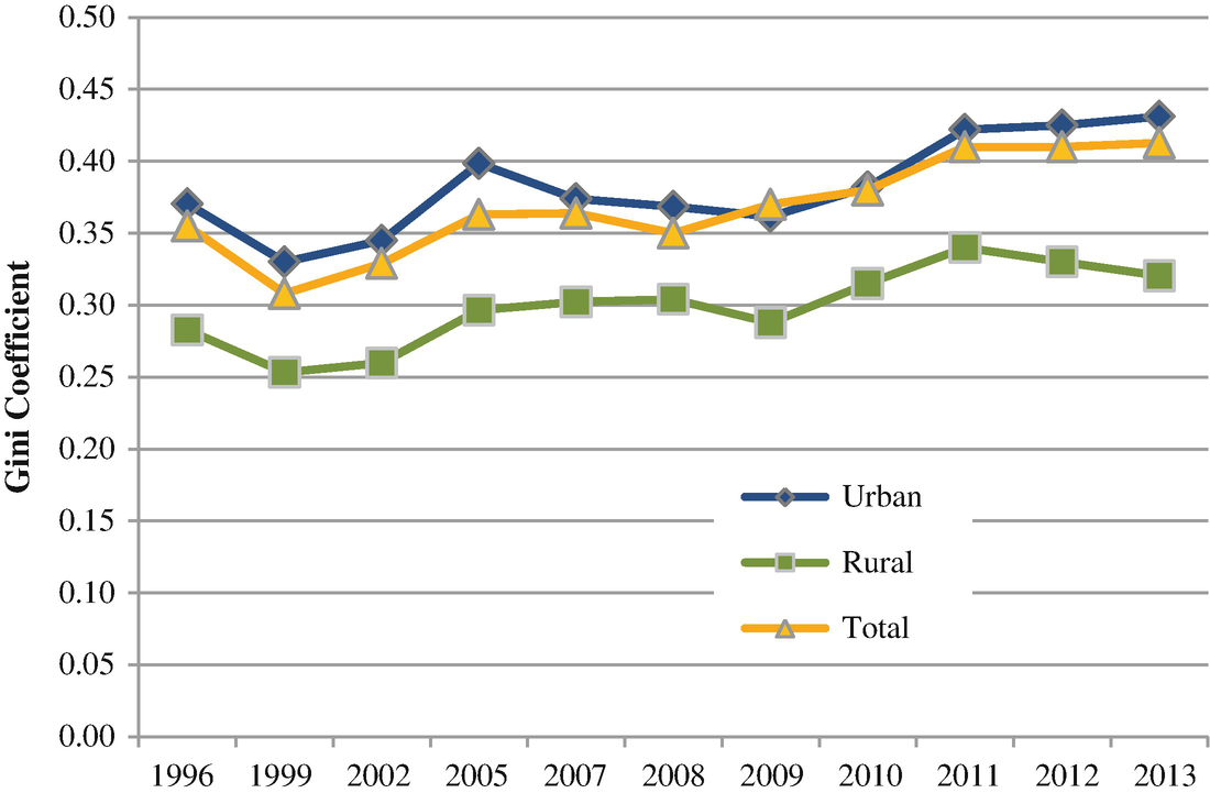
Figure 3.2 shows the trend of Gini coefficients over the period 1996–2013. While poverty has been declining over this time, it is clear that there has been a tendency for inequality to be increasing during this period. This is a national phenomenon across urban and rural areas (Miranti et al. 2013; Yusuf et al. 2014).

../images/457499_1_En_3_Chapter/457499_1_En_3_Fig2_HTML.png — Fig. 3.2
Trend in inequality, 1996–2013. (Source: SUSENAS, various years)

Figure 3.2 also shows that urban inequality is mirroring total inequality and inequality has been rising faster in urban than in rural areas (which in fact experienced a decline during 2011–2013).² This may be due to the increasing wages of the formal sector, which affects the top of the income distribution, as there has been increasing demand for skilled workers and consequently the presence of a skill premium. In contrast, at the bottom of the income distribution, the slow growth in the blue-collar workers has hindered the increase in wages among the poor (Manning and Miranti 2015). Further, wages in the agricultural sector in rural areas have also remained flat, particularly during the past decade, contributing to the gap between urban and rural areas.

In terms of regional inequality based on the latest data we have in 2013, surprisingly, provinces with high urban and total inequality are located in Sulawesi. Indeed, all of these five provinces are in the top 10 of provinces with high urban and total inequality. It is not surprising that DKI Jakarta, the capital city, records high inequality (see Table 3.2). Nevertheless, these provinces (and also West Java) have experienced a lower increase in inequality per year at 0.8% compared with other provinces in the top 10 that record more than 1.3% increase in the Gini index per year.

Table 3.2

The top 10 provinces with high urban and total inequality

Rank in 2013	Province	Gini index 1996		Gini index 2013		Change per year (%)
Rank in 2013	Province	Urban	Total	Urban	Total	Urban	Total
1	Southeast Sulawesi	0.34	0.32	0.46	0.43	2.01	1.82
2	DI Yogyakarta	0.36	0.36	0.45	0.44	1.33	1.21
3	Central Sulawesi	0.31	0.31	0.45	0.41	2.40	1.72
4	South Sulawesi	0.32	0.33	0.44	0.43	2.16	1.63
5	West Kalimantan	0.29	0.31	0.44	0.40	2.99	1.57
6	DKI Jakarta	0.38	0.38	0.43	0.43	0.82	0.82
7	Bengkulu	0.28	0.28	0.43	0.39	3.04	2.01
8	West Sulawesi			0.43	0.35
9	North Sulawesi	0.32	0.35	0.42	0.42	1.73	1.11
10	West Java	0.37	0.36	0.42	0.41	0.82	0.71
	Indonesia	0.37	0.36	0.43	0.41	0.91	0.76

Source: BPS, SUSENAS, various years

2.3 Urbanization

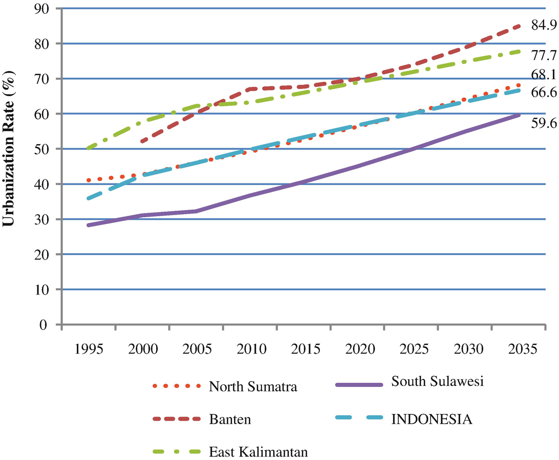
The speed of urbanization in Indonesia has been fast. By 2010, almost half of the population in Indonesia lived in urban areas, and it is predicted to increase to two-thirds of the population by 2035. Figure 3.3 shows that North Sumatra and Banten (which are included in the RUMiI data) have recorded high urbanization rates, which are higher than the national average and are expected to reach an urbanization rate of around 60% or more by 2035.³

../images/457499_1_En_3_Chapter/457499_1_En_3_Fig3_HTML.png — Fig. 3.3
Trend in urbanization, 1995–2035. (Source: BPS)
Note: Figures for 2015–2035 are predicted figures

Skeldon (1990, 1997) has proposed six stages of mobility transition when analyzing the migration pattern in developing countries. A pre-transitional society is followed by early transitional and then intermediate transitional, late transitional, early advanced, advanced, and, finally, late advanced society. Chotib (2002) has argued that if the urbanization rate has achieved 50%, this means the area has been close to the early advanced society. Looking at the data in 2010, Indonesia may have been close to the stage of early advanced society. Further, Table 3.3 displays the top 10 provinces with high urbanization rates. There are three main observations: (i) the high urbanization areas are concentrated in Western Indonesia, particularly in Java and Sumatra provinces, with the exception of East Kalimantan; (ii) the urbanization rate is very high—with the top 7 recording more than 60% urbanization rates; and (iii) three of the top 10 provinces are new provinces that were formed after the decentralization period.

Table 3.3

The top 10 provinces with high urbanization rate

Rank in 2010	Province	1995	2010	Change p.a. (%)
1	DKI Jakarta	100	100	0.00
2	Riau Islands		82.8
3	Banten		67
4	DI Yogyakarta	58.05	66.4	0.96
5	West Java	42.69	65.7	3.59
6	East Kalimantan	50.22	63.2	1.72
7	Bali	34.31	60.2	5.03
8	North Sumatra	41.09	49.2	1.32
9	Bangka Belitung		49.2
10	East Java	27.43	47.6	4.90
	Indonesia	35.91	49.8	2.58

Source: BPS

Nevertheless, one should keep in mind that there are three factors that influence urbanization. They are natural population increase, rural–urban migration, and reclassification (Firman et al. 2007; Gardiner 1997). In the case of Indonesia, it is important to take into account the reclassification of rural to urban areas as Gardiner (1997) explained that reclassification contributed to the high urban growth rate of 35% in 1980–1990.

2.4 Internal Migration

The most common type of internal migration discussed in the literature is rural–urban migration and interprovincial migration. Due to the nonavailability of long series rural–urban migration data, this subsection only discusses interprovincial migration.

The literature has discussed several types of migration based on reasons for migrating in Indonesia. The types of migration basically cover (i) economic-induced migration, (ii) education-induced migration, and (iii) migration for social and cultural reasons (see, e.g., Miranti 2007, 2013 for more details on interprovincial migration).

Figure 3.4 shows a comparison of the net interprovincial migration rates for 1995 and 2010. Positive net migration happens when in-migration to a province is higher than out-migration from that particular province, while negative out-migration is recorded when out-migration is higher than in-migration. Ordering the provinces based on the rank of net migration rates in 2010, the Outer Islands or Eastern Indonesia provinces mostly recorded a positive net migration rate, with an increase in the rate compared with that in 1995. These include the rich natural resource provinces such as East Kalimantan, Riau, and Aceh, which attract relatively more skilled migrants to the extraction and processing sites of natural resources such as oil and gas, other minerals, and palm oil. People also moved to the more sparsely populated Outer Islands such as Kalimantan because of the rapid development of the palm oil sector, which was labor-intensive and provided employment opportunities (Casson 2000).

../images/457499_1_En_3_Chapter/457499_1_En_3_Fig4_HTML.png — Fig. 3.4
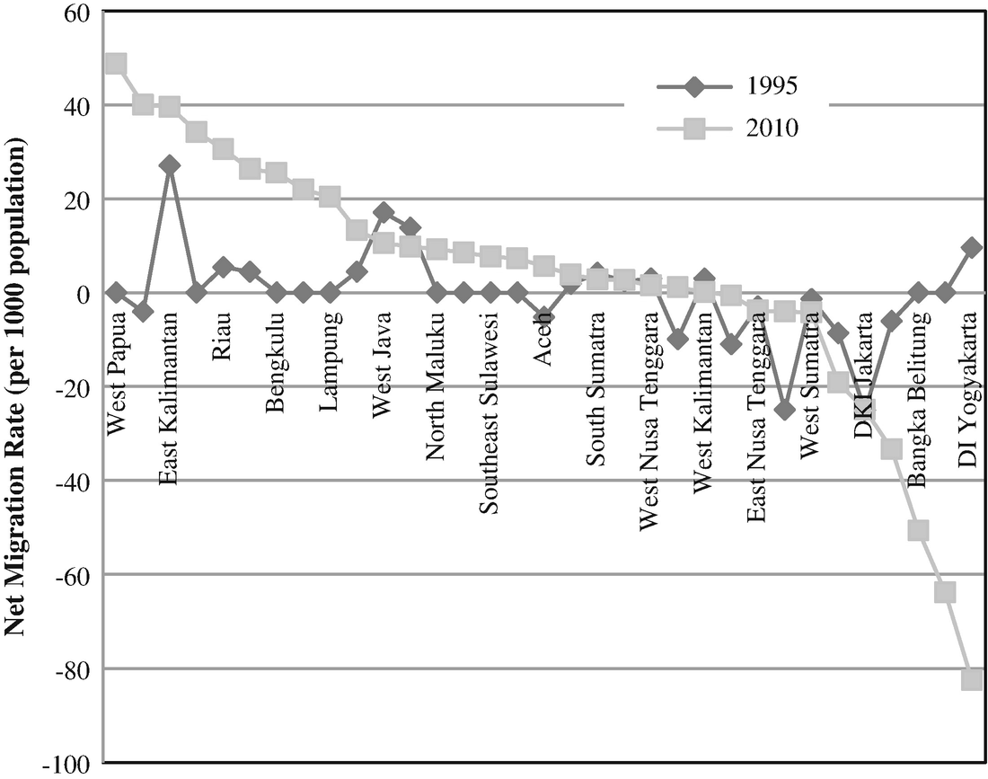
Net interprovincial migration rates (per 1000 population), 1995–2010. (Source: Indonesian Population Census 2010 and Intercensal Census 1995)

Jakarta recorded a negative net migration rate, which indicates the mobility of people who moved to West Java, especially to the nearby municipalities (Bogor, Tangerang, and Bekasi) but still commute to Jakarta to work. It is also interesting to observe that Yogyakarta, which is famously called a student city (Kota Pelajar), recorded negative net migration. Yogyakarta also ranks among the top 10 provinces with urban poverty, urban inequality, and high urbanization rates.

The preceding discussions reveal some interesting patterns and potential linkages between urbanization, urban poverty, urban inequality, and internal migration resulting from the development process.

3 Literature Review

To understand the link between poverty, inequality, urbanization, and internal migration, one should understand the determinants and factors associated with each of the variables and whether the links between each of the variables have been discussed in the literature.

The literature on the determinants of poverty, including empirical studies, has been abundant (see the literature review in Miranti 2007). It includes discussions on the impact of economic growth on poverty and the links between poverty and inequality.

Ravallion et al. (2007) have also studied the links between urbanization and claimed that urbanization is important for poverty reduction. Christiaensen et al. (2013) further proposed the mechanisms by which urbanization affects the speed of poverty reduction, which is not necessarily limited to urban poverty. These mechanisms are as follows. First, it is through the process of agglomeration economies that urban concentration can create economic growth and employment. Second, through the role of externalities, the production network is located close to not only its suppliers but also service providers and consumers. Third, rural off-farm employment facilitates the flow of inputs, goods, and services with urban areas, potentially contributing to declining poverty in rural areas. Fourth, remittances through urbanization (via rural–urban migration) play a potentially effective role in poverty reduction.

On reverse causality, the theory on the relationship between urbanization and economic development has been well developed. This includes the seminal chapter of Kuznets’ (1955) theory. Sagala et al. (2014) examine the link between urbanization and expenditure inequality in Indonesia using SUSENAS data to test the Kuznets hypothesis. They find that the inverted U-shaped hypothesis exists in both of their inequality estimates measured by the Theil index and the Gini coefficient. They also argue that inequality will reach its peak at an urbanization rate of around 46–50%. As urbanization rate in Indonesia has achieved 50%, this means that Indonesia has achieved the peak urbanization rate.

On the other hand, to the best of our knowledge, the discussion on the determinants of urbanization has been limited. For example, Hofmann and Wan (2013) focused on the potential impact of the growth of per capita GDP , structural transformation (industrialization), and knowledge spillovers (education) in determining urbanization. Applying OLS estimation using cross-country data and acknowledging the potential dual causality between urbanization and GDP growth, they find that the direction of effect is more likely from economic growth to urbanization rather than the opposite, as has been proposed by the World Bank and IMF (2013). They also find a positive impact of education on the urbanization rate and a significant positive impact of industrialization (measured by the proportion of nonagriculture to the total GDP) on urbanization. Firman et al. (2007) also argue that the services sector, which tends to be concentrated in large cities, is the driving factor behind urbanization and economic development as the growth of this service sector is supported by the availability of urban utilities such as water supply and electricity.

Having discussed urbanization, what does the literature say about migration or population mobility? The push–pull migration model in the neoclassical theory of migration argues that labor mobility aims to improve income and wealth and that it is a selective process (Sjaastad 1962; Greenwood 1975). The two most significant reasons for the decision to migrate are the income differential between the area of origin and area of destination and also the interaction of these with individual demographic and socioeconomic characteristics such as age, gender, and education (Harris and Todaro 1970; Fields 1982). However, the decision to migrate has since shifted to the family (Mincer 1978), and migration is also considered as human capital migration (Schultz 1961; Becker 1962). Recent literature has extended migration studies within the context of social capital (de Haas 2010).

Miranti (2007, 2010) has argued that the link between migration and poverty is ambiguous and depends on the role of the labor market. Using the example of interprovincial migration in Indonesia, she differentiates the roles of in-migration and out-migration in relation to poverty, directly or indirectly through economic growth, as follows:

In-migration (potential impact on the destination provinces)
- Direct effect. In-migration is expected to have a negative association with poverty if migrants have a higher educational level than the population in the destination region and, therefore, they have a higher opportunity of working in activities that give higher returns.
- Indirect effect. The assumption is that in-migration augments labor supply with increasing capital or/and human capital in destination areas and, therefore, migration contributes to economic growth in these regions, which is, in turn, negatively associated with poverty.
Out-migration (potential impact on the origin provinces)
- Direct effect. Out-migration is expected to have a positive relationship with poverty if out-migrants usually have higher educational levels than the population in the areas of origin and, therefore, a higher income status than those who remain behind.
- Indirect effect. The assumption is that migration contracts the labor supply because of a brain drain, but the possible offsetting impact of remittances contributes to an ambiguous impact from out-migration on growth in the regions of origin.

Further, Van Lottum and Marks (2012) have estimated the determinants of internal migration in Indonesia using a longer time series data spanning 1930–2000. By applying a gravity model, they find the capital city of Jakarta has a strong impact on the direction and the size of migration flows, while, in contrast, the wage differentials between the original and destination provinces are not significant.

At the level of micro-data analysis, in line with the literature that discusses migration as a family or household decision, the literature has highlighted the interplay between migration status, individual characteristics, household characteristics, and residential characteristics with poverty and other socioeconomic and well-being measures (see, e.g., Meng et al. 2010 for the Rural–Urban Migration project in the PRC and Indonesia).

4 Data, Approach, and Methodology

Two approaches are adopted in the analysis in this chapter. First, the quantitative analysis of the relationship between the poverty, inequality, urbanization, and internal migration in Indonesia uses RUMiI data, which is part of the output of the Rural–Urban Migration in China and Indonesia (RUMiCI) project hosted by the Australian National University (ANU). The data is longitudinal, conducted through four waves (2008, 2009, 2010, and 2011), and surveyed in four provinces in Indonesia that recorded major enclaves of rural–urban migrants. These provinces are North Sumatra, Banten, East Kalimantan, and South Sulawesi.⁴ Rural–urban migrants or the migration status is differentiated into (i) recent migrant (less than 5 years), (ii) long-term migrant (at least 5 years), and (iii) local nonmigrants.

The advantage of using this micro-data is that it allows the analysis of diversity of internal migrants and the changes in their well-being. Nevertheless, at this stage, for the purpose of this chapter, utilizing the longitudinal characteristic of the data may not be necessary, and instead the focus was on the early wave in 2008 where the economic situation was considered normal with no major economic shocks. The level of inequality proxied by the Gini coefficient in this particular year was also stable, while it started increasing in 2009 and reached 0.41 in 2011. Two regressions using the logit econometric technique are carried out to estimate (i) the likelihood to be in the bottom 20% of expenditure per capita and (ii) the top 20% of expenditure per capita (from relative poverty–inequality point of view) at the household level. This is in line with the literature which argues that migration is a household decision. Resosudarmo et al. (2010) have estimated the likelihood of being poor defined using absolute poverty line and probit model on the same dataset. A slightly different technique—the logit model—which may be easier to interpret is used. More detailed explanatory variables in the estimation, such as labor market industry and status, and include housing conditions to represent access to basic facilities/infrastructure, are incorporated.

Urbanization/internal migration are proxied by the migration status in the RUMiI data. Other explanatory variables include the demographic characteristics of the household heads, labor market characteristics of the household heads (industry and employment status), and housing condition (sanitation). The marginal effects of the variables of interest from these regressions are estimated and presented in the next section.

The second quantitative analysis of the relationship between urban poverty, urban inequality, urbanization, and internal migration in Indonesia uses panel data at the provincial level from 1995 to 2010. The dependent variable of the main equation is urban poverty. At this macro-level analysis, interprovincial migration data as proxy of internal migration is used since the rural–urban migration data is not available. The urbanization and interprovincial migration data are sourced from SUPAS 1995 and 2005 and the Indonesian Population Census 2000 and 2010, while urban poverty and urban inequality data are more frequently calculated based on the three yearly consumption modules of the household SUSENAS survey_.⁵ Therefore, we can only include the 2010 data as the latest data for the analysis. The discussion on migration will only be limited to recent migration, which covers those whose current residence is different from their place of residence 5 years ago.

Other data collection is sourced from the Indonesia BPS (Badan Pusat Statistik) , including data taken from SAKERNAS (labor force survey) and Statistics Indonesia. In addition, some assembled data from the CEIC Indonesia Premium Database is also included.

Taking into account the high degree of heterogeneity across provinces in Indonesia, it is therefore important that an econometric technique for panel data is applied. The data is constructed as an unbalanced panel due to, first, some missing values—a result of the creation of new provinces, particularly after the application of the decentralization policy in 2001. In 1995, there were 26 provinces, which expanded to 33 provinces by 2010. Second, the data is unbalanced because, SUSENAS being the main source of data for urban mean expenditure per capita , data was not collected in several provinces due to social conflicts or natural disasters (such as the tsunami in Aceh).

Urbanization is measured by the proportion of population living in urban areas, and the regressions also include other explanatory variables discussed in the literature to be associated with poverty. The best, suitable, and available proxy for each variable is chosen. These variables particularly include the role of the labor market such as provincial minimum wages; provision of physical infrastructure, which is proxied by percentage of households with state electricity (which could also represent the energy access) and education status of the population (educational attainment or net enrollment ratios at junior high school level); the size of the agricultural sector; and economic growth. Since this data is not published with urban–rural disaggregation, this limitation needs to be kept in mind when interpreting the results. Other variables were also considered important, but they could not be included in the analysis due to data unavailability. These include climate impact and data on wage disparities/convergence. There are also other limitations to the data including the fact that urbanization may increase as a result of changing classification from rural to urban areas as discussed earlier. The short panel data may also not be able to fully capture the interdependencies properly.

4.1 Empirical Models of Interdependencies

Since the focus of the chapter is the interdependencies between urban poverty, urban inequality, urbanization, and internal provincial migration, the estimations are carried out by acknowledging the dual causality between urban poverty as the dependent variable and urban inequality, urbanization, and internal provincial migration (and economic growth) as the endogenous variables, with other variables assumed as exogenous. Our hypothesis is that dual causality between these four key variables is present as indicated in Fig. 3.5.

../images/457499_1_En_3_Chapter/457499_1_En_3_Fig5_HTML.png — Fig. 3.5
Potential interdependencies between urban poverty, urbanization, urban inequality, and internal migration. (Source: Author’s summary)

We aim to carefully examine the interdependencies with simultaneous equations, in which each estimation will give the relative responsiveness of each variable to the other variables. However, we start with the simple panel data first without acknowledging the interdependency issue.⁶

Without interdependencies: These regressions are estimated separately using either the fixed effects or the random effects estimation of panel data .

1.
Urban poverty equation

$\begin{array}{l}\ln \kern0.5em urban povert{y}_{i,t}={\gamma}_0+{\gamma}_1\ln \kern0.5em urban gin{i}_{i,t}+{\gamma}_2 prop\_ urba{n}_{i,t}+{\gamma}_3 netmig\_ rat{e}_{i,t}\\ {}+\kern0.5em {\gamma}_4 economi{c}_{-} growt{h}_{i,t}+{\gamma}_5\ln \kern0.5em urban\exp \_ ca{p}_{i,t}+{\gamma}_6 prop\_ electricit{y}_{i,t}\\ {}+{\gamma}_7\ln \min \_ wag{e}_{i,t}+{\gamma}_8\ln \kern0.5em ner\_ junhig{h}_{i,t}+{\delta}_i+{\varepsilon}_{i,t}\end{array}$

2.
Urban inequality equation

$\begin{array}{l}\ln urban gin{i}_{i,t}={\beta}_0+{\beta}_1\ln urban povert{y}_{i,t}+{\beta}_2 prop\_ urba{n}_{i,t}+{\beta}_3 ne\mathit{\hslash nig}\_ rat{e}_{i,t}+\\ {}{\beta}_4 economic\_ growt{h}_{i,t}+{\beta}_5\ln urban\exp \_ ca{p}_{i,t}+{\beta}_6 prop\_ electricit{y}_{i,t}\\ {}+{\beta}_7\ln \min \_ wag{e}_{i,t}+{\beta}_8\ln ner\_ junhig{h}_{i,t}+{\beta}_9 non\_ agri+{\delta}_i+{\varepsilon}_{i,t}\end{array}$

3.
Urbanization equation

$\begin{array}{l} prop\_ urba{n}_{i,t}={\lambda}_0+{\lambda}_1\ln urban poven{y}_{i,t}+{\lambda}_2\ln urban gin{i}_{i,t}+{\lambda}_3 netmig\_ rat{e}_{i,t}\\ {}+{\lambda}_4 economic\_ gowt{h}_{i,t}+{\lambda}_5\ln urban\exp \_ ca{p}_{i,t}+{\lambda}_6 prop\_ electricit{y}_{i,t}\\ {}+{\lambda}_7\ln \min \_ wag{e}_{i,t}+{\lambda}_8\ln ner\_ junhig{h}_{i,t}+{\lambda}_9 no{n}_{-} agri+{\delta}_i+{\varepsilon}_{i,t}\end{array}$

4.
Interprovincial migration equation

$\begin{array}{l} netmig\_ rat{e}_{i,t}={\rho}_0+{\rho}_1\ln urban povert{y}_{i,t}+{\rho}_2\ln urban gin{i}_{i,t}+{\rho}_3 prop\_ urba{n}_{i,t}\\ {}+\kern0.5em {\rho}_4 economic\_ gowth+{\rho}_5\ln urban\exp \_ ca{p}_{i,t}+{\rho}_6 prop\_ electricit{y}_{i,t}\\ {}+{\rho}_7\ln {\min}_{-} wag{e}_{i,t}+{\rho}_8\ln ner\_ junhig{h}_{i,t}+{\rho}_9 non\_ agri+{\delta}_i+{\varepsilon}_{i,t}\end{array}$

With interdependencies: We carefully examined various strategies to achieve the best estimation, investigating whether the interdependencies between urban poverty and particularly urban inequality, urbanization, and internal migration exist. The main argument in this chapter can be summarized as follows: whether each of the variables of interest affects each other simultaneously. To incorporate dual causality into the model, we use the instrumental variable estimation technique, in which the 5-year lag of the endogenous variables and the 5-year lag of the incidence of urban poverty are used as the instruments for the first-step estimations. As the literature also indicates that economic growth affects poverty reduction and vice versa, we also include this as the endogenous variable. Size of the nonagricultural sector is included as an additional instrument, particularly to represent the degree of structural transformation in each province, which the literature points out is associated with urbanization. We assume that the instruments are not correlated with the error terms in the main equation as the instruments used also include 5-year lags of the endogenous variables. Due to the nature of the data, which covers only a short period, time dummy variables are not included in the analysis as they are highly correlated with the explanatory variables.

We use panel data estimation, fixed effects, or generalized least squares random effects—two-stage least squares—and use the Hausman test to decide the preference.

5.
Urban inequality equation

$\begin{array}{l}\ln urban gin{i}_{i,t}={\eta}_0+{\eta}_1 lag\ln urban poven{y}_{i,t-5}+{\eta}_2 lagprop\_ urba{n}_{i,t-5}\\ {}+{\eta}_3 lagnetmig\_ rat{e}_{r-5}+{\eta}_4 lageconomic\_ growt{h}_{t-5}+{\eta}_5 non\_ agr{i}_{t-5}\\ {}\begin{array}{l}+{\eta}_6\ln urban\exp \_ ca{p}_{i,t}+{\eta}_7 prop\_ electricit{y}_{i,t}+{\eta}_8\ln \min \_ wag{e}_{i,t}\\ {}+{\eta}_9\ln ner\_ junhig{h}_{i,t}+{\eta}_{10} lag\ln urban gin{i}_{i,t}+{\delta}_i+{\varepsilon}_{i,t}\end{array}\end{array}$

6.
Urbanization equation

$\begin{array}{l} pro{p}_{-} urba{n}_{i,t}={\sigma}_0+{\sigma}_1 lag\ln urban poven{y}_{i,t-5}+{\sigma}_2 lagprop\_ urba{n}_{i,t-5}\\ {}+{\sigma}_3 lagnetmi{g}_{-} rat{e}_{r-5}+{\sigma}_4 lageconomic\_ growt{h}_{t-5}+{\sigma}_5 non\_ agr{i}_{t-5}\\ {}\begin{array}{l}+{\sigma}_6\ln urban\exp \_ ca{p}_{i,t}+{\sigma}_7 prop\_ electricit{y}_{i,t}+{\sigma}_8\ln \min \_ wag{e}_{i,t}\\ {}+{\sigma}_9\ln ner\_ junhig{h}_{i,t}+{\sigma}_{10} lag\ln urban gin{i}_{i,t}+{\delta}_i+{\varepsilon}_{i,t}\end{array}\end{array}$

7.
Interprovincial migration equation

$\begin{array}{l} netmig\_ rat{e}_{i,t}={\beta}_0+{\beta}_1 lag\ln urban poven{y}_{i,t-5}+{\beta}_2 lagprop\_ urba{n}_{i,t-5}\\ {}+{\beta}_3 lagnetmig\_ rat{e}_{r-5}+{\beta}_4 lageconomic\_ growt{h}_{t-5}+{\beta}_5 non\_ agr{i}_{t-5}\\ {}\begin{array}{l}+{\beta}_6\ln urban\exp \_ ca{p}_{i,t}+{\beta}_7 prop\_ electricit{y}_{i,t}+{\beta}_8\ln \min \_ wag{e}_{i,t}\\ {}+{\beta}_9\ln ner\_ junhig{h}_{i,t}+{\beta}_{10} lag\ln urban gin{i}_{i,t}{\delta}_i+{\varepsilon}_{i,t}\end{array}\end{array}$

8.
Economic growth equation

$\begin{array}{l} economic\_ growt{h}_{i,t}={\rho}_0+{\rho}_1 lag\ln urban povert{y}_{i,t-5}+{\rho}_2 lagprop\_ urba{n}_{i,t-5}\\ {}+{\rho}_3 lagnetmig\_ rat{e}_{r-5}+{\rho}_4 lageconomic\_ growt{h}_{t-5}+{\rho}_5 non\_ agr{i}_{t-5}\\ {}\begin{array}{l}+{\rho}_6\ln urban\exp \_ ca{p}_{i,t}+{\rho}_7 prop\_ electricit{y}_{i,t}+{\rho}_8\ln \min \_ wag{e}_{i,t}\\ {}+{\rho}_9\ln ner\_ junhig{h}_{i,t}+{\rho}_{10} lag\ln urban gin{i}_{i,t}+{\delta}_i+{\varepsilon}_{i,t}\end{array}\end{array}$

The main equation used here is the reduced form of the modified estimation (Ravallion and Chen 1997; Adams and Page 2003, 2005). This is also an extension of Miranti et al. (2013) and Miranti et al. (2014), which estimate the growth elasticity of poverty in Indonesia using panel data at the provincial level (1984–2010) with provincial poverty as the dependent variable.

9.
Urban poverty equation

$\begin{array}{l}\ln urban povert{y}_{i,t}={\gamma}_0+{\gamma}_1\ln urban gin{i}_{i,t}+{\gamma}_2 prop\_ urba{n}_{i,t}+{\gamma}_3 netmig\_ rate+\\ {}{\gamma}_4 economic\_ growth+{\gamma}_5\ln urban\exp \_ cap+{\gamma}_6 prop\_ electricity\\ {}+{\gamma}_7\ln \min \_ wage+{\gamma}_8\ln ner\_ junhigh+{\delta}_i+{\varepsilon}_{i,t}\end{array}$

where

i is province.
t is year (1995, 2000, 2005, and 2010).
urbanpoverty is the urban poverty incidence (%).
urbangini is the urban Gini coefficient.
prop_urban is the proportion of urban population (%).
netmig_rate is the rate of net migration (in-migration – out-migration) per 1000 population.
economic_growth is the annual economic growth of regional gross domestic product (RGDP) per capita (%).
urbanexp_cap is the urban expenditure per capita (IDR).
prop_electricity is the proportion of household with state electricity subscription (%).
min_wage is the provincial minimum wage (IDR).
ner_junhigh is the net enrollment ratio for junior high school (%).
non_agri is the proportion of nonagricultural RGDP to total RGDP (%).
δ is provincial fixed effects.
ε is random errors.

5 Estimation Results

5.1 Findings from Household Data Analysis

The estimated marginal effects of the explanatory variables of probability of being in the bottom 20% or top 20% of household per capita expenditure are shown in Table 3.4. The bottom 20% and top 20% are calculated on the basis of the distribution of yearly household per capita expenditure. Some important findings are as follows.

Table 3.4

Findings of RUMiI data

		Probability of being in the bottom 20%			Probability of being in the top 20%
		Marginal effect	Std. error	Sig	Marginal effect	Std. error	Sig
		(1)	(2)	(3)	(4)	(5)	(6)
Head of household demographic characteristics
Female headed		0.015	0.029		−0.003	0.022
Age		−0.002	0.001	*	0.004	0.001	***
Number of children		0.025	0.004	***	−0.027	0.006	***
Education	(Base: no schooling)
	Did not complete the primary	−0.016	0.031		−0.112	0.022	***
	Primary school	−0.048	0.026	*	−0.083	0.024	***
	Junior high school	−0.069	0.024	***	−0.030	0.028
	Senior high school	−0.118	0.025	***	0.024	0.029
	Diploma	−0.138	0.016	***	0.121	0.064	*
	Bachelor’s degree and above	−0.132	0.016	***	0.154	0.055	***
Marital status	(Base: single)
	Married	0.145	0.027		−0.295	0.041	***
	Divorce/widow	0.281	0.081	*	−0.115	0.018	***
Head of household labor market characteristics
Industry	(Base: manufacturing)
	Construction	0.074	0.038	*	−0.056	0.030	*
	Finance	0.153	0.118		0.079	0.087
	Real estate	0.143	0.158		0.008	0.114
	Education and health	0.003	0.047		0.034	0.042
	Trade, service, and others	0.025	0.021		−0.027	0.021
Employment status (Base: not working)
	Employee	0.030	0.029		0.031	0.028
	Civil service or military	−0.094	0.029	***	0.121	0.062	**
	Self-employee/unpaid	−0.028	0.029		0.111	0.040	***

Source: Author’s calculation from RUMiI data

Note: Significance at the 1%, 5%, and 10% levels is denoted by ***, **, and *, respectively

		Probability of being in the bottom 20%			Probability of being in the top 20%
		Marginal effect	Std. error	Sig	Marginal effect	Std. error	Sig
		(1)	(2)	(3)	(4)	(5)	(6)
Migration status (Base: local, not migrant)
	Recent migrant	−0.114	0.020	***	0.049	0.028	*
	Long-term migrant	−0.042	0.015	***	0.010	0.018
Housing condition—sanitation (Base: no sanitation)
	Have toilet and bathroom	−0.141	0.065	**	0.067	0.060
	Have either toilet or bathroom	−0.022	0.048		−0.026	0.076
	Public toilet	−0.049	0.042		0.011	0.082
Number of observation		2426			2426
Log likelihood		−1052.724			−1024.280
Pseudo R²		0.135			0.155
Marginal effects after logit		0.154			0.152

Source: Author’s calculation from RUMiI data

Note: Significance at the 1%, 5%, and 10% levels is denoted by ***, **, and *, respectively

5.1.1 Migration Status

Table 3.4 shows that after controlling for individual and household characteristics and compared to the local population or nonmigrants, the migration status (particularly for the recent migrants) has a significant effect in determining the likelihood of being in the bottom quintile and top quintile. Being a recent migrant has a higher marginal effect in reducing the probability of being in the bottom 20% than the long-term migrant. The likelihood of being in the bottom 20% of household expenditure is reduced by 11.4 percentage points for a recent migrant and around 4.2 percentage points for a long-term migrant compared to the nonmigrants. The finding for recent migrants indicates those migrants have better socioeconomic status than the nonmigrants, which may refer to the fact that migration is indeed selective. Effendi et al. (2010a, b) find that recent migrants consist of younger individuals with better education. Compared to the nonmigrants and holding other variables constant, the impact of being a recent migrant is significant and increases the likelihood of being in the top of the expenditure distribution by five percentage points.

5.1.2 Head of Household/Demographic Characteristics

It seems the number of children—that is, the number of dependents in a household—is a significant determinant and increases the likelihood of being in the bottom quintile of household expenditure. Age has a significant and negative association with the likelihood of being in the bottom 20% and increases the likelihood of being in the top 20%. This may indicate that the older the age, the more capable/experienced the person is to explore various opportunities to increase the likelihood of their household living in a better socioeconomic condition. The impact of gender of the head of household is surprisingly not significant, while the impact of marital status is limited, with a divorcee/widow decreasing the likelihood of being in the top 20% by 11.5 percentage points, compared to a single person. Marriage is also negatively correlated with being in the top of the expenditure distribution, as compared to a single person; being married decreases the likelihood of being in the top 20% by almost 30 percentage points. The main message from the marriage variable is that a person who is single, or without any dependents, is more correlated with higher income/wealth.

Human capital is also an important determinant in comparison to those who do not have education. For example, having an educational attainment of a bachelor’s degree or above decreases the likelihood of being in the bottom quintile of household per capita expenditure by 13.2 percentage points compared to those who do not have education. The higher the level of educational attainment, the stronger these effects tend to be. The regression to estimate the likelihood of being in the top 20% indicates that the role of having tertiary education at the diploma level or bachelor’s degree and above is crucial.

5.1.3 Head of Household Labor Market Characteristics

The labor market effect is somewhat limited, with only working in the construction industry (compared to manufacturing) having a significant increase in the likelihood of being in the bottom quintile and reducing the likelihood of being in the top quintile. This indicates that having a blue-collar occupation is related to a higher likelihood of being at the bottom of the income distribution.

Based on the labor market status, the findings show that being a member of the civil services or military services is advantageous (compared to not working), which reduces the likelihood of being in the bottom quintile or increases the likelihood of being in the top quintile, other things held constant. Having an own business or family work significantly increases the likelihood of being in the top quintile (Appendix Table 3.8).

5.1.4 Housing Condition (Infrastructure)

We have chosen sanitation to represent the housing condition of the household as the other categories within this variable are mutually exclusive. As expected, compared to households that do not have sanitation facilities, living in households that have proper sanitation (e.g., toilet and bathroom) reduces the likelihood of being in the bottom quintile.

5.2 Findings from Macro-panel Data Analysis

Appendix Table 3.9 discusses the regression results for model (i), which has not acknowledged the interdependencies between the four variables.⁷ It is shown that there are some significant associations between the four variables. For example, interprovincial migration has a negative impact on urban inequality; urban inequality reduces interprovincial migration; urbanization significantly reduces urban poverty.

Tables 3.5 and 3.6 present the regression results for model (ii), which acknowledges the interdependencies. The result from the Hausman test indicates the preference to use random effects estimation rather than fixed effects. Table 3.5 displays the results from the first stage of the regressions, where the causality runs from the lag of the urban poverty incidence 5 years ago and other exogenous variables to the endogenous variables (urban inequality, urbanization, net interprovincial migration, and economic growth). Table 3.6 provides the second stage of the main equation, where the opposite causality runs from urban inequality, urbanization, net interprovincial migration, and economic growth to urban poverty.

Table 3.5

First-stage regressions—endogenous variables (random effect, 2SLS)

	Urban inequality			Urbanization			Net provincial migration			Economic growth
	Coef.	Std.	Sig.	Coef.	Std.	Sig.	Coef.	Std.	Sig.	Coef.	Std.	Sig.
lnurbanexp_cap	0.185	0.067	***	8.937	2.813	***	−3.198	13.046		2.269	2.319
prop_electricity	0.002	0.002		0.200	0.066	***	−0.200	0.308		0.105	0.055	*
lnmin_wage	−0.038	0.063		−8.521	2.645	***	4.428	12.268		−1.188	2.181
lnner_junhigh	0.158	0.142		2.107	5.959		−6.517	27.640		5.509	4.914
lag lnurbangini	−0.270	0.092	***	-13.438	3.888	***	10.257	18.031		−0.614	3.206
lag prop_urban	0.002	0.002		0.510	0.074	***	−0.392	0.341		−0.132	0.061	**
lag netmig_rate	2.278E-04	0.001		−7.824E-03	0.022		−4.119E-01	0.103	***	5.667E-03	0.018
lag economic growth	−2.626E-04	0.001		0.028	0.031		−0.125	0.144		−0.194	0.026	****
prop non_agri to GDP	−0.003	0.003		0.412	0.123	***	0.104	0.571		−0.024	0.101
lag lnurbanpov_rate	0.057	0.031	*	−0.279	1.320		−0.509	6.121		−1.268	1.088
constant	−4.366	0.661	***	−109.372	27.775	***	74.792	128.819		−39.512	22.902	*

Source: Author’s calculation

Note: Significance at the 1%, 5%, and 10% levels is denoted by ***, **, and *, respectively

Table 3.6

Main equation

	Urban poverty
	Coef.	Std. err.	Sig.
lnurbangini	1.488	0.817	*
prop_urban	−0.016	0.008	**
netmig_rate	1.796E-04	0.004
economic growth	−0.014	0.012
lnurbanexp_cap	−0.654	0.303	**
prop_electricity	0.000	0.006	***
lnmin_wage	−0.050	0.229
lnner_junhigh	0.697	0.529
constant	10.470	4.354	**
sigma_u	0.407
sigma_e	0.204
rho	0.799
R²: within	0.687
between	0.587
overall	0.586
N	69

Source: Author’s calculation

Note: Significance at the 1%, 5%, and 10% levels are denoted by ***, **, and *, respectively

The results of the first-stage regressions show that, as expected, the lags of the explanatory variables have significant impacts on their respective contemporaneous dependent variables (see Table 3.5). Urban inequality is positively affected by urban mean expenditure per capita and the 5-year lag of the urban poverty rate, which is expected. Although there is a positive impact of urbanization on urban inequality, the impact is not significant. The higher the expenditure per capita of urban population on average, the higher is the inequality. The results of the coefficient of lag of urban poverty rate 5 years ago mean that higher poverty rates in the past should be translated to higher effort required to improve the welfare of people living in the bottom quintile of income distribution, and if the other part of the distribution does not change, this may increase inequality.

We also examine variables that explain urbanization and find that there are significant and positive impacts of urban mean expenditure per capita , access to electricity, and the proportion of nonagricultural sector to the GDP. These associations are expected as urbanization would increase when a province is more developed with higher income and better access to infrastructure and when the development of the nonagricultural sector (which supports the finding from Hofmann and Wan 2013) or formal employment also happens. Minimum wage is surprisingly found to reduce urbanization. Increasing the minimum wage to protect employees and increase their well-being may hinder formal employment in the urban areas when it is set above the market wage and creates unemployment, as indicated in the Harris–Todaro model. This is particularly true for Indonesia, where the application of a minimum wage potentially has an adverse impact on employment in the urban labor-intensive manufacturing sector. Further, despite minimum wages having increased by around 6.5% per year between 2000 and 2010, the effect has been limited, and it is not beneficial for those who are in the bottom of the wage distribution. Not to mention that an increase in the minimum wage is usually also followed by increases in commodity prices, which does not improve workers’ consumption (Bird and Manning 2008). If this is happening, it is not surprising that it has impeded the urbanization process.

The net migration equation surprisingly shows that only the lag of the net migration variable is significant. The finding from the economic growth equation that urbanization has a negative association with economic growth is also somewhat surprising. An increase in the urbanization rate by 1 percentage point reduces economic growth by 0.13 percentage point. This may be the result of the short panel data we have used in estimating the model or the fact that the urbanization rate has reached 50%, meaning it may have reached its peak so that economic growth may experience diminishing returns despite urbanization. Further investigation is required on this aspect. It is surprising that the education variable is not significant in all specifications that may indicate the limitation of the data we use—that is, the net enrollment ratio for junior high school. This variable may not capture the variation within provinces as Indonesia adopts the policy of 9 years of schooling. It is expected that the results would be better if we use the net enrollment ratio for the senior high school level. However, the longer time series of enrollment ratio data for secondary high school is not available. We have also used the educational attainment data, which does not improve the regression results.

Table 3.6 shows further findings from the main equation, which examines the reverse causality from the endogenous explanatory variables on urban poverty and the impacts on poverty of the other exogenous variables, which are the urban expenditure per capita , access to electricity, minimum wage, and net enrollment ratio at the junior high school and equivalent level. As expected, the results show that 1% increase in urban inequality measured by the Gini index will contribute to around 1.5% increase in urban poverty rate, while a 1% increase in the mean expenditure of the urban population will contribute to 0.7% decline in the urban poverty rate. Inequality has hampered the impact of the increase of average expenditure to the poverty rate. The rate of urbanization is poverty reducing in urban areas. It is interesting that the coefficient of better facilities and infrastructure, as indicated by electricity, while significant at 1%, is really marginal, being close to zero.

Table 3.7 provides the summary of the results from the aggregate/macroanalysis, which shows that interdependencies do indeed exist but mostly in the form of single direction causality. Dual causality has been only found in the relationship between urban poverty and inequality.

Table 3.7

Summary of interdependencies

Dual causality
Urban poverty		Urban inequality
Single causality
Urbanization		Urban poverty
Urban inequality		Urbanization
Urban mean expenditure per capita		Urban poverty
Urban mean expenditure per capita		Urban inequality
Urban mean expenditure per capita		Urbanization
Minimum wage		Urbanization
Proportion of electricity		Urban poverty
Proportion of electricity		Economic growth
Proportion of nonagricultural sector to GDP		Urbanization

Source: Author’s summary

6 Conclusion and Policy Recommendations

This chapter investigates the issues and interdependencies of urbanization, internal migration, urban poverty, and urban inequality in Indonesia. There are two key objectives of the chapter. First, in the microanalysis, the focus is on examining the determinants of the likelihood of being in relative poverty (the bottom versus the top expenditure quintile). Second, the macroanalysis examines the determinants of urban poverty by taking into account the potential interdependencies between urban poverty, urbanization, internal migration, and urban inequality.

The results from microanalysis using rural–urban migration data in Indonesia (RUMiI), which test the determinants of the likelihood of being in the bottom 20% and top 20% of expenditure distribution, show the importance of migration status and various demographic and socioeconomic characteristics as the explanatory variables. These include age, number of children, education, marital status, and labor market characteristics. The results from macro−/aggregate analysis using panel data of provinces in Indonesia from 1995 to 2005 show that the presence of causality is mostly in the form of a single causality, except the dual causality that exists between urban poverty and urban inequality.

The findings from both the macro- and microanalyses, if not supporting each other, are complementary. The link between micro- and macroanalysis is present from the analysis, particularly on two main points. First, the finding that urbanization is poverty reducing (from the macroanalysis) has been supported by the finding that rural–urban migration (measured by migration status), which is one of the determinants of urbanization, has an impact on reducing the likelihood of being in the bottom 20%. Second, both the macro- and microanalyses support the importance of the provision and access to basic facilities or infrastructure as a strategy to reduce poverty. The results from the housing (sanitation) condition from the microanalysis and the proportion of households with electricity from the macroanalysis support this conclusion. However, it looks like the channel at the aggregate level is indirect, which is from electricity, which significantly increases urbanization, which in turn reduces the rate of urban poverty.

With microanalysis, the results provide more evidence from the labor market perspective that the two measures used in the analysis—that is, industry of work and employment status—have some effect on the likelihood of being in the bottom or top 20% of the distribution. In contrast, the impact of minimum wage is not significant in the macroanalysis, whereas that of education is also captured by the microanalysis but not the macroanalysis.

We conclude that interdependencies do exist between the four variables, but they are complex. Given these results, our question is: what are the strategies and policy recommendations to jointly manage the interdependencies among the elements of the internal migration–urbanization–poverty–inequality nexus in Indonesia? First, the dual causality between urban poverty and urban inequality suggests that policies should aim to reduce not only poverty but also inequality. Policies to reduce inequality are back on the table for discussion, after many concerns have been raised on the increasing inequality experienced by this country. Efforts are required to not only improve the welfare of the bottom 20% of the population, which includes those who are poor, but also have more equalizing fiscal policy and tax reforms to ensure the redistribution from the top 20% of population. Second, urbanization through rural–urban migration is poverty reducing since migrants who move to urban areas are usually the young and the more educated. The implication of this is the need for better formal job opportunities being made available in the urban areas for absorbing these workers. This will be a challenge because previous data suggest that job seekers are never fully absorbed into the labor market, given the number of vacancies available to those seeking employment. Thus, incentives should be offered to various business/investment opportunities to create more jobs in urban areas and to reduce barriers to labor market entry. Third, the importance of education and availability of good infrastructure, in terms of access to electricity and good sanitation, are also very important. These will improve the quality of life of the rural–urban migrants and link them with employment, trade activities, further education, and other activities. More expenditure directed toward this should be recommended.

The views expressed in this publication are those of the authors and do not necessarily reflect the views and policies of the Asian Development Bank (ADB) or its Board of Governors or the governments they represent.

ADB does not guarantee the accuracy of the data included in this publication and accepts no responsibility for any consequence of their use. The mention of specific companies or products of manufacturers does not imply that they are endorsed or recommended by ADB in preference to others of a similar nature that are not mentioned.

By making any designation of or reference to a particular territory or geographic area, or by using the term "country" in this document, ADB does not intend to make any judgments as to the legal or other status of any territory or area.

Open AccessThis work is available under the Creative Commons Attribution-NonCommercial 3.0 IGO license (CC BY-NC 3.0 IGO)http://creativecommons.org/licenses/by-nc/3.0/igo/. By using the content of this publication, you agree to be bound by the terms of this license. For attribution and permissions, please read the provisions and terms of use at https://www.adb.org/terms-use#openaccess.

This CC license does not apply to non-ADB copyright materials in this publication. If the material is attributed to another source, please contact the copyright owner or publisher of that source for permission to reproduce it. ADB cannot be held liable for any claims that arise as a result of your use of the material. Please contact pubsmarketing@adb.org if you have questions or comments with respect to content, or if you wish to obtain copyright permission for your intended use that does not fall within these terms, or for permission to use the ADB logo.

Appendix

Table 3.8

Correlation coefficient

Variables	urbanpov_rate	urbangini	urban	netmig_rate	Economic growth	urbanexp_cap	prop_electricity	min_wage	ner_junhigh	prop non_agri to GDP
urbanpov_rate	1
urbangini	−0.03	1.00
urban	−0.35	0.33	1.00
netmig_rate	−0.13	−0.21	−0.19	1.00
economic growth	0.09	0.11	−0.05	0.00	1.00
urbanexp_cap	−0.46	0.44	0.32	0.03	−0.10	1.00
prop_electricity	−0.16	0.40	0.71	−0.19	−0.05	0.36	1.00
min_wage	−0.42	0.36	0.19	0.05	−0.10	0.94	0.29	1.00
ner_junhigh	−0.14	0.33	0.57	−0.13	−0.17	0.45	0.72	0.41	1.00
prop non_agri to GDP	−0.39	0.10	0.79	−0.02	−0.13	0.19	0.54	0.12	0.36	1

Source: Author’s summary

Table 3.9

Independent estimations

	Urban inequality			Urbanization			Net provincial migration
	Coef.	Std.	Sig.	Coef.	Std.	Sig.	Coef.	Std.	Sig.
lnp0	0.029	0.027		0.239	1.592		−4.557	5.307
lnurbangini				1.661	5.036		−35.443	17.070	**
prop_urban	0.002	0.002					−0.354	0.329
netmig_rate	−1.011E-03	0.001	*	−0.022	0.031
economic growth	0.002	0.001	**	0.020	0.041		0.363	0.143	***
lnurbanexp_cap	0.109	0.070		11.272	3.260	***	1.436	12.106
prop_electricity	0.001	0.001		0.236	0.068	***	−0.172	0.233
prop non_agri	−0.001	0.002		0.776	0.120	***	0.299	0.453
lnmin_wage	−0.011	0.066		−9.828	3.055	***	1.811	11.285
lnner_junhigh	−0.105	0.098		3.142	5.267		25.056	17.929
constant	−2.118	0.619	***	−130.741	30.679	***	−156.560	114.283
sigma_u	0.047			7.287			20.530
sigma_e	0.096			3.771			15.654
rho	0.197			0.789			0.632
R²:
within	0.400			0.598			0.123
between	0.229			0.791			0.137
overall	0.391			0.777			0.110

Source: Author’s calculation

Note: Significance at the 1%, 5%, and 10% levels is denoted by ***, **, and *, respectively

	Urban poverty
	Coef.	Std. err.	Sig.
lnurbangini	−0.047	0.361
prop_urban	−0.017	0.005	***
netmig_rate	−0.002	0.002
economic growth	0.002	0.003
lnurbanexp_cap	−0.110	0.242
prop_electricity	0.005	0.005
lnmin_wage	−0.249	0.229
lnner_junhigh	1.012	0.357	***
constant	1.327	2.043
sigma_u	0.367
sigma_e	0.318
rho	0.572
R²: within	0.347
between	0.387
overall	0.382
N	103

Source: Author’s calculation

Note: Significance at the 1%, 5%, and 10% levels is denoted by ***, **, and *, respectively

References

Adams Jr., R. H., & Page, J. (2005). Do international migration and remittances reduce poverty in developing countries. World Development, 33(10), 1645–1669.
Adams Jr., R. H., & Page, J. (2003). International migration, remittances, and poverty in developing countries (The World Bank Policy Research Working Paper 3179).
Becker, G. S. (1962). Investment in human capital. Journal of Political Economy, 70(5), 9–49.
Bird, K., & Manning, C. (2008). Minimum wages and poverty in a developing country: Simulations from Indonesia’s household survey. World Development, 36(5), 916–933.
Casson, A. (2000). The hesitant boom: Indonesia’s oil palm sub-sector in an era of economic crisis and political change (No. 29). Bogor: Center for International Forestry Research.
Chotib. (2002). Urbanisasi Tidak Selalu Berkonotasi Negatif. Warta Demografi, 4(32), 55–63.
Christiaensen, L., Weerdt, J., & Todo, Y. (2013). Urbanization and poverty reduction: The role of rural diversification and secondary towns. Agricultural Economics, 44(4–5), 435–447.
de Haas, H. (2010). Migration and development: A theoretical perspective. International Migration Review, 44(1), 227–264.
Effendi, T. N., Mujiyani, F. I., Darmawan, D. A., & Widhyarto, D. S. (2010a). Assessing the welfare of migrant and non-migrant households in four Indonesia cities: Some demographic, social and employment characteristics. In X. Meng, C. Manning, L. Shi, & T. N. Effendi (Eds.), The great migration: Rural-urban migration in China and Indonesia (pp. 153–197). Northampton: Edward Elgar Publishing.
Effendi, T. N., Mujiyani, F. I., Darmawan, D. A., & Widhyharto, D. S. (2010b). Assessing the welfare of migrant and non-migrant households in four Indonesian cities: Some demographic, social and employment characteristics. In X. Meng, C. Manning, L. Shi, & T. N. Effendi (Eds.), The great migration: Rural-urban migration in China and Indonesia (pp. 153–177). Northampton: Edward Elgar Publishing.
Fields, G. S. (1982). Place-to-place migration in Colombia. Economic Development and Cultural Change, 30(3), 539–558.
Firman, T. (2004). Demographic and spatial patterns of Indonesia’s recent urbanization. Population, Space and Place, 10(6), 421–434.
Firman, T., Kombaitan, B., & Pradono, P. (2007). The dynamics of Indonesia’s urbanization, 1980–2006. Urban Policy and Research, 25(4), 433–454.
Gardiner, P. (1997). Migration and urbanization: A discussion. In Indonesia assessment: Population and human resources (pp. 118–133). Canberra: Australian National University.
Greenwood, M. J. (1975). Research on internal migration in the United States: A survey. Journal of Economic Literature, 13(2), 397–433.
Harris, J. R., & Todaro, M. P. (1970). Migration, unemployment and development: A two-sector analysis. The American Economic Review, 60(1), 126–142.
Hofmann, A., & Wan, G. H. (2013). Determinants of urbanization (ADB Working Chapter Series, No. 355). Manila: Asian Development Bank.
Kuznets, S. (1955). Economic growth and income inequality. American Economic Review, 45, 1–28.
Manning, C., & Miranti, R. (2015). The SBY legacy on jobs, poverty and income distribution: A mixed record. In E. Aspinall, M. Mietzner, & D. Tomsa (Eds.), The Yudhoyono years: An assessment. Singapore: Institute of Southeast Asian Studies.
Manning, C., & Sumarto, S. (2011). Employment, living standards and poverty: Trends, policies and interactions. In C. Manning & S. Sumarto (Eds.), Employment, living standards and poverty in contemporary Indonesia. Singapore: Institute of Southeast Asian Studies.
Meng, X., Manning, C., Shi, L., & Effendi, T. N. (2010). The great migration: Rural-urban migration in China and Indonesia. Northampton: Edward Elgar Publishing.
Mincer, J. (1978). Family migration decisions. Journal of Political Economy, 86(5), 749–773.
Miranti, R. (2007). The determinants of regional poverty in Indonesia:1984–2002. PhD thesis, Australian National University.
Miranti, R. (2010). Poverty in Indonesia 1984–2002: The impact of growth and changes in inequality. Bulletin of Indonesian Economics Studies, 46(1), 79–97.
Miranti, R. (2013). Provincial poverty rates in Indonesia, 2006–2011. Report prepared for the TNP2K, Support for Economic Analysis Development in Indonesia (SEADI), USAID.
Miranti, R., Vidyattama, Y., Hansnata, E., Cassells, R., & Duncan, A. (2013). Trends in poverty and inequality in decentralising Indonesia (OECD Social, Employment and Migration Working Chapters, No. 148). OECD Publishing.
Miranti, R., Duncan, A., & Cassells, R. (2014). Revisiting the impact of consumption growth and inequality on poverty in Indonesia during the decentralisation period. Bulletin of Indonesia Economic Studies, 50(3), 461–482.
Ravallion, M., & Chen, S. (1997). What can new survey data tell us about recent changes in distribution and poverty ? World Bank Economic Review, 11(2), 357–382.
Ravallion, M., Chen, S., & Sangraula, P. (2007). New evidence on the urbanization of global poverty. Population and Development Review, 33(4), 667–701.
Resosudarmo, B. P., Suryahadi, A., Purnagunawan, R. M., Yumna, A., & Yusrina, A. (2010). The socio-economic and health status of rural-urban migrants in Indonesia. In X. Meng, C. Manning, L. Shi, & T. N. Effendi (Eds.), The great migration: Rural-urban migration in China and Indonesia (pp. 178–193). Northampton: Edward Elgar Publishing.
Sagala, P., Akita, T., & Yusuf, A. A. (2014). Urbanization and expenditure inequality in Indonesia: Testing the Kuznets hypothesis with provincial panel data. Letters in Spatial and Resource Sciences, 7(3), 1–15.
Schultz, T. W. (1961). Investment in human capital. The American Economic Review, 51(1), 1–17.
Sjaastad, L. A. (1962). The costs and returns of human migration. Journal of Political Economy, 70(5), 80–93.
Skeldon, R. (1990). Population mobility in developing countries. London/New York: Belhaven Press.
Skeldon, R. (1997). Of migration, great cities, and markets: Global systems of development. In W. Gungwu (Ed.), Global history and migrations (pp. 183–215). Boulder: Westview Press.
The World Bank and International Monetary Fund. (2013). Global monitoring report 2013: Monitoring the MDGs.
Van Lottum, J., & Marks, D. (2012). The determinants of internal migration in a developing country: Quantitative evidence for Indonesia, 1930–2000. Applied Economics, 44(34), 4485–4494.
Yusuf, A. A., Sumner, A., & Rum, I. A. (2014). Twenty years of expenditure inequality in Indonesia 1993–2013. Bulletin of Indonesia Economic Studies, 50(2), 243–254.

Footnotes

There are three types of migration or population mobility that are usually a focus of the literature, rural–rural, rural–urban, and international migration, although urban–urban and urban–rural migrations are also worthy topics for discussion.

World Bank (2013) and Manning and Miranti (2015) have argued that several factors are behind this increasing inequality, including fiscal policy, which has been less equalizing in comparison with other countries.

The BPS (1980, 1990, and 2000) defines an Indonesian locality as urban if it fulfills the following characteristics: “(i) having a population density of 5000 people or more per square kilometer; (ii) having 25% or less of households working in the agricultural sector; (iii) having eight or more kinds of urban facilities”(Firman 2004, p. 425).

These locations should be kept in mind when interpreting the findings.

Some are calculated by special data request from the Indonesia BPS.

We also try the Arellano–Bond estimation using the xtabond2, which is suitable for analysis of dynamic panel data with small T but larger N. However, our data is too short for this type of estimation for three reasons. First, we will lose much information due to the inclusion of lags. Second, there is also a requirement to limit the number of endogenous variables to be less than the total observations in each group. Third, the Arellano–Bond estimation does not provide the results of the first stage of the equation, so it does not reveal the interdependencies.

Table A1 presents the correlation coefficient between the variables.