Let's assume that you are tracking the financial records of your company and your boss wants you to deliver two reports every week, containing the total amount of sales that you made for a particular week and the total amount of purchases you made toward the company's stores. How would you go about it?
You can always select all of the instances of sales and then calculate the sum of them. Once that is done, you have to again select all instances of purchases made and find the sum of purchases too. Having to do so frequently would be really time-consuming and boring. Here's where the CHOOSE function comes into play! We can implement a simple model that does everything for you in one click, using the following steps:
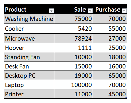
- Load all of the required values that you need to account for and compile them into a table, as seen here:
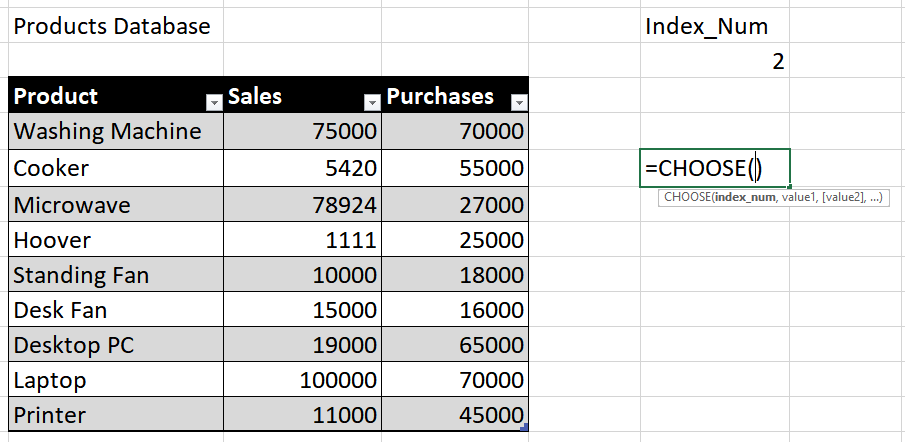
- We will now start writing the CHOOSE function:
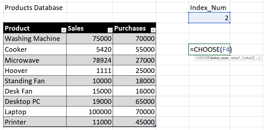
- The first value we need to enter is the cell where we have put the options, which, in our case, is F4:
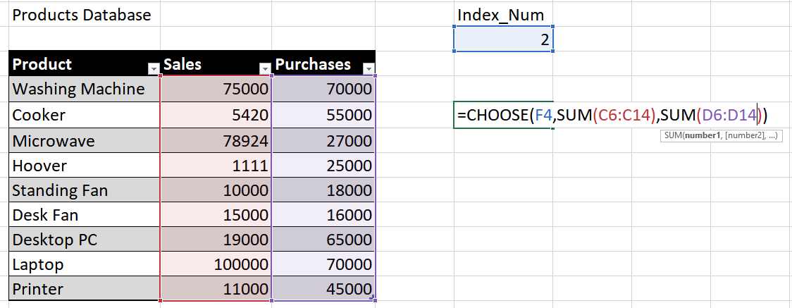
- Now, we will assign two options to F4, 1 and 2, using data validation. We will now edit the formula so that if we select 1, the cell where the formula is input will display the sum of all of the sales made for that week, and if we select 2, it will display the sum of all of the purchases. So, first we will select all of the cells in the Sales column, C6 to C14, and input it into the formula cell as SUM(C6:C14), as seen here:

- Next, we will select all of the cells in the Purchases column and input those into the next field of the formula as SUM(D6:D14), as follows:
- This results in the following output:
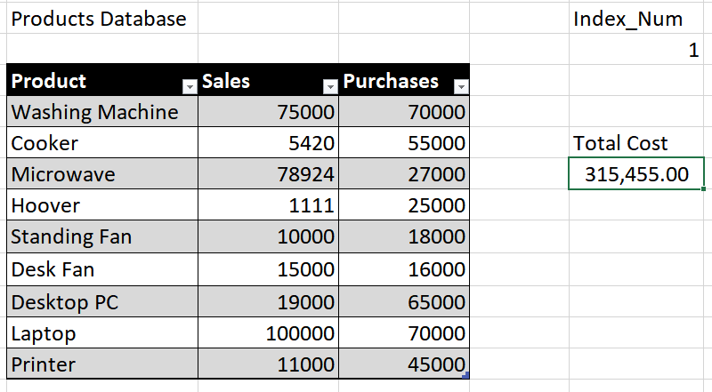
Now, as seen in the preceding screenshot, when 1 is selected, the cost of sales becomes visible, which, in our case, is 315,455.00.
- If we select 2, we will get the cost of purchases, as seen here:

This is just a basic scenario in which the function can come in handy. This will be particularly useful when you have large amounts of data that needs to be filtered and sorted.