To avoid the aforementioned shortcomings, you should enter the cell references of the cells containing the values, rather than typing the actual values, as shown in the following screenshot:
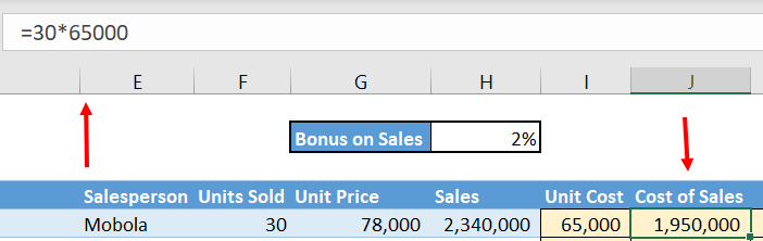
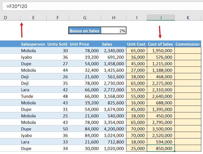
The formula bar in the preceding screenshot shows that we entered F5*I5.
In this way, it is clear where the input is coming from. All the cells that have formulas that refer to those cells will be automatically updated.
Another advantage of referencing is that, by default, Excel registers the position of the cell references relative to the active cell. So, in the preceding example, F5 is registered as four cells to the left, and I5 is registered as one cell to the left of the active cell, J5.
The relevance of this is that, when you copy that formula to another location, Excel remembers the positions of the original cell references included in the formula, relative to the original active cell. Excel then adjusts the references accordingly in order to maintain those positions relative to the new active cell.
So, if the formula is copied 15 cells down, the row part of the reference is adjusted by 15 rows down, and so F5*I5 automatically becomes F20*I20. In this way, since the formula is the same, that is, Units Sold × Unit Cost, we can simply copy our formula down the list and still obtain the correct answers. This can be seen in the following screenshot:
This technique of referencing the cells, instead of their actual values, is called relative referencing.
There are several different ways to copy to a range of cells, which are as follows:
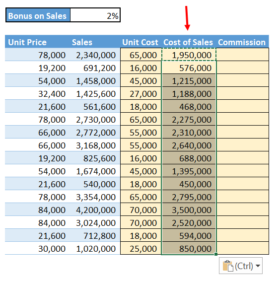
- The first way is to select the cell or range of cells to be copied, press Ctrl + C, select the range of cells to which you are going to copy, and then press Enter or Ctrl + V.
If you press Ctrl + V, Excel places a Ctrl icon at the bottom right of the last cell of the range. You can then click on the icon or simply press Ctrl and a box of Paste Special options will appear, as shown in the following screenshot:
You can then select, paste format, paste values, transpose, or perform any one of the other options.
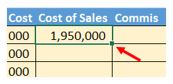
- The second way is built into Excel. There is a small black box that appears at the bottom right of the selected cell, called the fill handle. When you hover the cursor over the fill handle, it turns into a thick black cross. Select the cell with the value to be copied, and then hold the right mouse button down on the fill handle and drag it down the range of cells that you want to copy. Then, release the right mouse button. The following screenshot shows the fill handle of a cell in Excel:
- Alternatively, you could just double-click on the fill handle and all the cells below, up to the last row of the table. These will be filled by the original cell. You don't need to preselect the cells—all you need to do is press Ctrl + C for this method to work.
However, the cells in the adjacent column, left or right, must be populated in order to indicate to Excel how far down you wish to fill the formula.
- The last way to do this is as follows—starting with and including the cell with the formula to be copied, select the range of cells to be copied to, and then press Ctrl + D. All the cells that are selected will be populated with the formula. This method is my personal favorite and, along with double-clicking the fill handle, is the most elegant way to copy to a range of cells. You could also use this method to fill to the right by pressing Ctrl + R. You will find this very useful for filling formulas to the right, across the columns of the forecast years in your financial model.