In this section, we will explore grid searches.
We'll talk a bit about optimization versus grid searching, setting up a model generator function, setting up a parameter grid and doing a grid search with cross-validation, and finally, reporting the outcomes of our grid search so we can pick the best model.
So why, fundamentally, are there two different kinds of machine learning activities here? Well, optimization solves for parameters with feedback from a loss function: it's highly optimized. Specifically, a solver doesn't have to try every parameter value in order to work. It uses a mathematical relationship with partial derivatives in order to move along what is called a gradient. This lets it go essentially downhill mathematically to find the right answer.
Grid searching isn't quite so smart. In fact, it's completely brute force. When we talk about doing a grid search, we are actually talking about exploring every possible combination of parameter values. The grid search comes from the fact that the two different sets of parameters forms a checkerboard or grid, and the grid search involves running the values that are in every square. So, as you can see, grid searching is radically less efficient than optimization. So, why would you ever even use a grid search? Well, you use it when you need to learn parameters that cannot be solved by an optimizer, which is a common scenario in machine learning. Ideally, you'd have one algorithm that solves all parameters. However, no such algorithm is currently available.
Alright, let's look at some code:
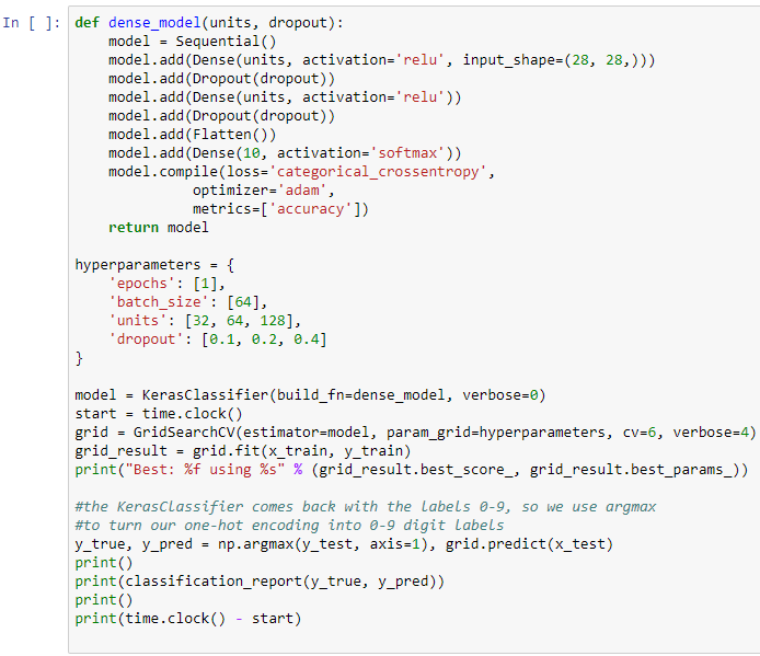
We're going to be using scikit-learn, a toolkit often used with Keras and other machine learning software in order to do our grid search and our classification report, which will tell us about our best model. Then, we're also going to import Keras's KerasClassifier wrapper, which makes it compatible with scikit_learn.
So now, let's focus on a model-generating function and conceive two hyperparameters. One of them will be dropout and the other one will be the number of units in each one of the dense hidden layers. So, we're building a function here called dense_model that takes units and dropout and then computes our network as we did previously. But instead of having a hard-coded 32 or 0.1 (for example), the actual parameters are going to be passed in, which is going to compile the model for us, and then return that model as an output. This time, we're using the sequential model. Previously, when we used the Keras functional model, we chained our layers together one after the other. With the sequential model, it's a lot more like a list: you start off with the sequential model and you add layer after layer, until the sequential model itself forms the chain for you. And now for the hyperparameter grid. This is where we point out some shortcomings of the grid search versus an optimizer. You can see the values we're picking in the preceding screenshot. We'll do one epoch in order to make things run faster, and we'll keep a constant batch_size of 64 images that will vary between 32, 64, and 128 hidden units, and dropouts of 0.1, 0.2, and 0.4. Here's the big shortcoming of grid search: the hyperparameters you see listed here are the only ones that will be done—the grid search won't explore hyperparameter values in-between.
Now, we set up our KerasClassifier, handing it the model-building function we just created and setting verbose to 0 to hide the progress bars of each Keras run. Then, we set up a timer; I want to know how long this is going to take. Now, we set up a grid search with cross-validation. For its estimator, we give it our model, which is our KerasClassifier wrapper, and our grid parameter (see the preceding hyperparameters), and we say cv=6, meaning cut the data (the training data) into six different segments and then cross-validate. Train on 5, and use one sixth to validate and iteratively repeat this in order to search for the best hyperparameter values. Also, set verbose to 4 so that we can see a lot of output. Now that much is running with Keras alone, we call the fit function going from our x training data (again, those are our input images) to our y training data (these are the labels from the digits zero to nine) and then print out our best results. Note that we haven't actually touched our testing data yet; we're going to use that in a moment to score the value of the best model reported by the grid search.
Now, we test the result. This is where we use argmax. Again, this is a function that looks into an array and picks out the index that has the largest value in it. Effectively, this turns an array of ten one-hot encoded values into a single number, which will be the digit that we're predicting. We then use a classification report that's going to print out x grid that shows us how often a digit was predicted correctly compared to the total number of digits that were to be predicted.
Alright, so the output of the preceding code is as follows:

We're exploring each of the parameters in the hyperparameter grid and printing out a score. This is how the grid search searches for the best available model. When we're all done, a single model will have been picked. In this case, it's the one with the largest number of hidden units, and we're going to evaluate how well this model is using our testing data with the classification report.
In the following screenshot, you can see that the printout has each one of the digits we've recognized, as well as the precision (the percentage of time that we correctly classified the digit) and the recall (the number of the digits that we actually recalled):

You can see that our score is decent: it's 96% accurate overall.