In this section, we're going to build a full convolutional neural network. We're going to cover the MNIST digits and transform that data to have channels construct the convolutional neural network with multiple layers, and then finally, run and train our convolutional neural network and see how it compares to the classical dense network.
Alright! Let's load up our MNIST digits, as shown in the following screenshot :

You can see that we're performing a similar operation to what we did for the dense neural network, except we're making a fundamental transformation to the data. Here, we're using NumPy's expand_dims call (again, passing -1, meaning the last dimension) to expand our image tensors from the 28 x 28 pixel MNIST images to actually have an additional dimension of one, which encodes the color. In this case, it's a black and white image, so it's a gray scale pixel; that information is now ready to use with the convolutional layers in Keras.
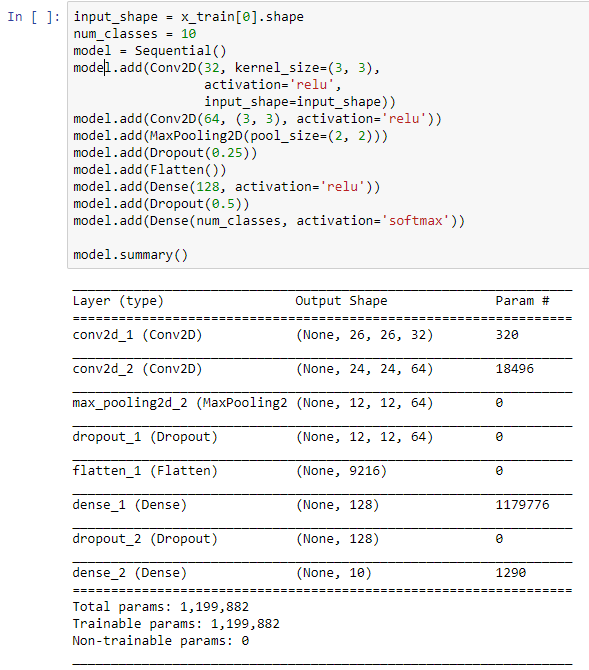
Alright, let's start adding our layers. The first thing we're going to do is put together a convolutional 2D layer with a kernel size of 3 x 3. This is going to slide a 3 x 3 pixel matrix over the image, convolving that down to a smaller number of outputs, and then handing it on to a secondary convolutional 2D layer, again with a 3 x 3 matrix. This, in a sense, serves to build an image pyramid. It reduces and focuses the data in the image to an ever smaller number of dimensions, and then we pass it through the max pooling, which reduces it further still.
Now, it's starting to look like our dense neural network from before. We perform a dropout in order to avoid overfitting; we flatten it to remove all the separate dimensions so that now, there's just one dimension left; and then we pass it through a dense neural network, before finally feeding it on to our friend, softmax, who, as you remember, will classify our digits from zero to nine, the individual written digits of zero through nine. That generates our final output:

Alright, so this is similar to a dense network in total structure, except we've added a preprocessing set of layers that do convolution.
Alright, let's give this thing a run!

As I mentioned previously, machine learning definitely involves human waiting, because we're going to run and train multiple layers. But you can see that the actual training code we run (the model compilation and the model fit) is the exact same as before from when we worked with the dense neural network. This is one of the benefits of Keras: the plumbing code to make it all go stays roughly the same and then you can change the architecture, putting in different layers, putting in different numbers of activations, or putting in different activation functions so that you can experiment with different network shapes that may work better with your individual set of data. In fact, you can experiment with the layer in this notebook. You can, for instance, change the activations from 32 and 64 to 64 and 128, or add in another dense layer before the final softmax output.
Now, running this training on your system, it might be time-consuming. On my machine, it took about 10 minutes to complete the entire set of training. But you'll notice right away that we're getting quite a bit better accuracy. If you cast your mind back to the last section, our dense neural network achieved an accuracy of about 96%. Our network here is a lot closer to 99%, so, by adding in convolutions, we've successfully built a much more accurate classifying neural network.