Now, we're going to create an actual deep neural network using convolution.
In this section, we'll cover how to check to make sure we're running on a GPU, which is an important performance tip. Then, we'll load up our image data, and then we'll build a multiple block deep neural network, which is much deeper than anything we've created before. Finally, we'll compare the results of this deep neural network with our shallow convolutional neural network in the previous section.
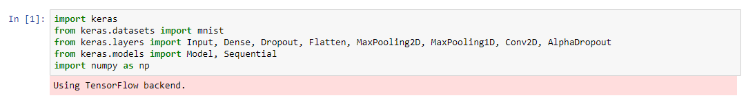
Here, at the top, we're importing the necessary Python packages:
This is the same as we did for the standard convolutional neural network. The difference regarding making a deep neural network is that we're simply going to be using the same layers even more. In this next block, we're going directly to tensorflow and importing the python library. What is this device_lib we're seeing? Well, device_lib actually lets us list all of the devices that we have access to in order to run our neural networks. In this case, I'm running it on an nvidia-docker setup and have access to the GPU, which will boost performance:

If you don't have a GPU, that's fine! Just know that it'll take materially longer (maybe as much as 20 times longer) to run these deep neural networks on a CPU setup. Here, we're importing the MNIST digit training data, the same as before:
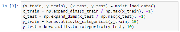
Remember that we're expanding the dimensions with the -1 (meaning that we're expanding the last dimension) to install channels, and we're normalizing this data with respect to the maximum value so that it's set up for learning the output values (the y values). Again, we switch them to categorical; there are ten different categories, each corresponding to the digits zero through nine.
Alright! Now, the thing that makes a deep neural network deep is a recurring series of layers. We say it's deep with respect to the number of layers. So, the networks we've been building previously have had one or two layers before a final output. The network we have here is going to have multiple layers arranged into blocks before a final output. Okay, looking at the first block:
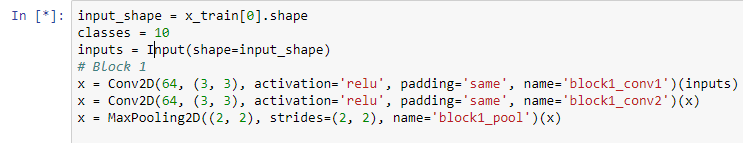
This actually forms a chain where we take a convolution of the inputs and then a convolution of that convolution, and then finally apply a max pooling in order to get the most important features. In this convolution, we're introducing a new parameter that we haven't used before: padding. In this case, we're padding it using same value, meaning we want the same amount of padding on all sides of the image. What this padding actually does is that when we convolve down, because of our 3 x 3 kernel size, the image ends up being, slightly smaller than the input image, so the padding places a perimeter of zeros on the edge of the image to fill in the space that we shrunk with respect to our convolution. Then, ending on the second block, you can see here that we switch from 64 activations to 128 as we attenuate the image:
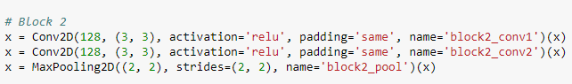
Essentially, we're shrinking down the image to a denser size, so we're going from 28 pixels by 28 pixels through this pooling layer of 2 x 2 down to 14 pixels by 14 pixels, but then we're going deeper in the number of hidden layers we're using to extrapolate new features. So, you can actually think of the image honestly as a kind of pyramid, where we start with the base image and stretch it out over convolution, and narrow it down by pooling, and then stretch it out with convolution, and narrow it down by pooling, until we arrive at a shape that's just a little bit bigger than our 10 output layers. Then, we make a softmax prediction in order to generate the final outcome. Finally, in the third block, very similar to the second block, we boost up to 256 hidden features:
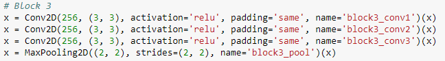
This is, again, stretching the image out and narrowing it down before we go to the final output classification layer where we use our good old friend, the dense neural network. We have two layers of dense encoding, which then ultimately go into a 10 output softmax.
So, you can see that a deep neural network is a combination of the convolutional neural network strung deeply together layer after layer, and then the dense neural network is used to generate the final output with softmax that we learned about in the previous sections. Let's give this thing a run!

Okay, you can see the model summary printing out all of the layers here, chained end-to-end with 3.1 million parameters to learn. This is by far the biggest network we've created so far.
Now, it's time to train this network on our sample data and see how well it predicts. Okay, we're training the model now, and it's going relatively quickly:
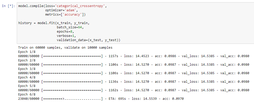
On my computer, getting through the iterations took about 3.5 minutes with my Titan X GPU, which is really about as fast as you can get things to go these days with a single GPU solution. As we get to the end of the training here, you can see that we have an accuracy of 0.993, which is 1/10 or 1% better than our flat convolutional neural network. This isn't that big of an improvement it seems, but it is definitely an improvement!
So, we'll now ask: why? Simply, past 99% accuracy, marginal improvements are very, very difficult. In order to move to ever higher levels of accuracy, substantially larger networks are created, and you're going to have to spend time tuning your hyperparameters. The examples we ran in this chapter are running more than eight epochs. However, we can also change the learning rates, play with the parameters, perform a grid search, or vary the number of features. I'll leave that to you as an experiment.