CHAPTER 2
EVA and Value
How does EVA determine a company’s share price? Not directly. It is not, after all, a per share measure. But EVA is the best measure of all to compute share prices and to explain actual stock price performance. If that were not true, there would be no case for EVA.
EVA ties to share prices indirectly through a sister measure that I call MVA, standing for market value added. As it turns out, MVA is far more significant than stock price itself. Here’s why. MVA is the dollar difference between the total cash that investors have put or left in a business, and which now stands on its balance sheet as its invested capital, and the present value of the cash that they can expect to take out of the business, as indicated by the firm’s share price. For example, if a company has a total market value or enterprise value of $1 billion, and has invested $600 million of capital in net business assets, then it has created MVA of $400 million, the difference.
As I said, this is a really important measure. It shows, first, how much wealth the firm has created for its owners by comparing what they have put in with what they can get out. Put another way, MVA is franchise value, the value of the business above just putting the assets in a pile. It is also, mathematically, the market’s assessment of the net present value (NPV) of all investments the company has made, those already in place plus those expected to materialize down the road. Put it all together, and MVA is more important than share price.
In fact, increasing MVA should be every company’s most important financial goal. An increase in MVA reveals, as no other measure can, how successful management had been at allocating, managing, and redeploying scarce resources of all kinds so as to maximize the wealth of the owners by maximizing the net present value of the enterprise. That being the case, every board and top team should track it.
As mentioned, EVA ties to share prices through its link to MVA. How important is that? It is all-important. That’s because EVA is the only performance measure that directly ties to MVA. The link between MVA and EVA exists because EVA also is the only measure that ties to NPV—to net present value. I call this the fundamental principle of wealth creation, and it states: The present value of a forecast for EVA is always mathematically identical to the net present value of discounted cash flow, or to what is the same thing, MVA at the corporate level. Why is that? By virtue of the capital charge, EVA sets aside the profit that must be earned to recover the value of the capital that has been or will be invested, and as a result, EVA always discounts to the net present value of a project or decision. It always discounts to the market value above the invested capital. And at the corporate level a forward plan projection of EVA always discounts to the consolidated company’s MVA. You will see an example of that in just a minute.
I say this with great conviction and emphasis because we have developed a software tool that automatically calculates NPV and MVA both ways, by discounting cash flow and by discounting the EVA, and it always produces the same answer for a given forecast. The equality I am stressing is not a theory or something you might or might not believe. It is a mathematical truth, just as 2 + 2 = 4. And as you will see later on, projecting and discounting EVA is at the heart of value-based planning and decision making.
Putting the math aside for a moment, consider the implications. If a company, a line of business, or a capital investment project is forecast to just break even on EVA—to just earn the cost of capital—then it breaks even on NPV. It will only be worth the book value of the capital invested in it. There is no NPV, no franchise value, no owners’ wealth, and no MVA without EVA. You can grow everything else. You can expand sales, earnings, EBITDA, and margins all you want. But if you are not growing EVA you are not creating value—you are at best only preserving it.
On the bright side, once EVA turns positive and a firm generates more profit with its capital than its investors could earn by investing it on their own, then value is being added, wealth created, and a real franchise value established. And the greater the EVA and the faster, surer, and longer it grows, the greater the NPV and MVA will be. This is why Fortune magazine dubbed EVA “the real key to creating wealth” in the cover story that introduced EVA to its readers in September 1993.
Let’s examine the EVA/MVA connection for Ball Corporation over the period from midyear 1997 to midyear 2012 as an example. The top chart in Exhibit 2.1 plots Ball’s market value as the light bar versus its capital as the dark bar. The spread between the two is MVA, the market value added to the capital, and it is shown on the bottom chart.
Exhibit 2.1 Ball Corporation’s Market Value, MVA, and EVA (dollars in millions)
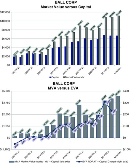
By market value I mean the total value the market is assigning to all the capital invested in the firm’s net business assets. It starts with the market capitalization of the common equity given the share price and also includes debt and other liabilities and the present value of rents on leased facilities and equipment, less excess cash. In other words, market value is what it would cost to buy the business, debt and rent free and free of excess cash, at prevailing market prices. Capital is the corresponding investment in the firm’s net business assets, including rented assets, and also net of excess cash, so that the two measures correspond, and MVA is simply the difference between the two.
Ball’s MVA is plotted as the ascending bar on the left scale in the lower chart, and the firm’s EVA profit is traced by the line on the right scale. MVA increased over the years because Ball’s market value generally increased by more than its capital increased. Ball added to the stock of its positive NPV investments, and as a result, Ball added to the stock of its owners’ wealth. As important, it added to its MVA by adding to its EVA. Ball’s MVA increased hand in hand with the demonstrated ability to earn and increase economic profit. As expected, EVA was indeed the key to creating wealth at Ball Corporation.
Let’s zoom in on details. In midyear 1997, Ball’s market value and its capital both stood at about $2 billion (top chart), and thus its MVA was virtually nil at a time when EVA was negative but beginning to improve (bottom chart). EVA rose fairly steadily and certainly impressively after that, reaching a peak of over $300 million for the four-quarter period ending in mid-2011. In response, starting from a standstill, Ball’s MVA ascended to a wealth premium that is now over $4 billion. Ball is thus a good example of how an EVA bonus plan forges a direct link between pay and value-adding performance.
Note, also, that Ball did not generate EVA and MVA by milking its business, but by nourishing growth. Management invested aggressively, as the firm’s capital base increased from about $2 billion in 1997 to nearly $6.5 billion 15 years later in order to expand its business globally and to consummate a number of important acquisitions.
In the most recent period, Ball’s EVA turned down somewhat and yet its MVA held up. Ball is in the process of an aggressive expansion campaign, and capital investment costs have temporarily depressed EVA. The market, though, has looked beyond that and is impounding the long-run expected stream of EVA into the current MVA. As an EVA company, Ball has earned a measure of credibility that enables it to make significant strategic investments while retaining investors’ confidence that management is batting with their interests in mind.
In case you suspect that Ball was simply surfing an EVA wave common to its industry, take a look at the EVA/MVA chart for Crown Holdings, a principal competitor in the metal can business (Exhibit 2.2). Without getting bogged down in the year-to-year details, the fact is that over the long term, Crown’s EVA has essentially moved sideways, and MVA as well. The picture is starkly different from Ball’s.
Exhibit 2.2 Crown Holdings’ Market Value, MVA, and EVA (dollars in millions)
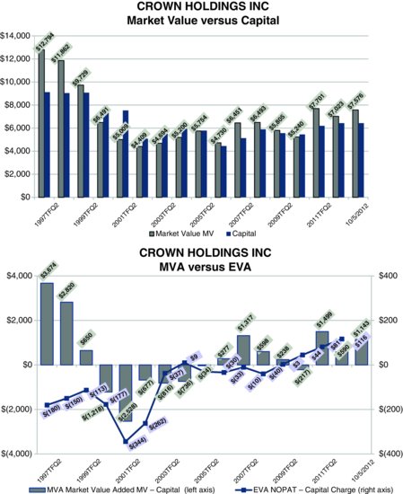
The two cases illustrate a general rule. In the real world, changes in MVA are best explained by changes in EVA, far better than measures like growth in sales, earnings or EBITDA, margins, and returns. EVA measures wealth creation, in principle and in practice. And as a result, managers can analyze, project, and discount EVA to measure NPV and owner wealth with the confidence that they are focusing on the measure that really matters and accurately simulating how the market will respond.
One company that does that is Volkswagen, which also makes Audi, Bentley, Bugatti, and Lamborghini branded vehicles, among others. The company’s financial management is governed by EVA. The criteria for new investments and initiatives is to approve only those where the NPV—as measured by the present value of the projected EVA—is positive after considering project-specific risks and company-wide consequences.
Managers, moreover, are instructed to improve and optimize NPV by improving the stream of EVA profit that the investment can be configured to generate. The procedure to do that is described in the firm’s EVA manual, an excerpt of which is shown in Exhibit 2.3. It shows that Volkswagen will forecast line-of-business net operating profit after taxes (NOPAT) and the charge for the incremental capital employed over the product life cycle, and then discount the resulting EVA at a 9 percent hurdle rate to measure net present value that is the basis for decision making. Incidentally, you can download a full PDF copy of the manual from the company’s website at www.volkswagenag.com/content/vwcorp/info_center/en/publications/2010/08/Finanzielle_Steuerungsgroessen.bin.html/binarystorageitem/file/Financial+Control+System+3e.pdf.
Exhibit 2.3 Volkswagen Financial Control System

As the Volkswagen example suggests, the present value of EVA is indeed identical to the net present value of discounted cash flow. I have said that is so because EVA sets aside the cost of capital needed to recover the value of the invested capital. But still, at a more fundamental level, why is the present value of a forecast for EVA always identical to discounted cash flow and NPV?
You can grasp it without a complicated proof. I like to put it in banking terms. Suppose I lend you $100 and then I say you have two choices. You can pay back the loan right away or you can take your time. Pay me back over 10 years, say, at a rate of $10 a year. As long as you pay me a market rate of interest on the unpaid loan balance, the present value of getting paid back right away and getting paid back over time with interest is exactly the same, by definition.
What is the analogy? The cash flow that is discounted to measure NPV is computed as if the loan was paid back right away. Investment spending is deducted from cash flow when it is forecast to be spent. EVA, on the other hand, is like paying the loan back over time, as assets are depreciated or charged through cost of goods sold and with a market rate of interest assessed on the outstanding loan balance. The present value is always the same, and regardless of the depreciation period chosen, from expensing right away to no depreciation at all to anything in between. This being the case, everything that validates cash flow or discounted cash flow as a management and valuation tool automatically validates EVA as well. Discard EVA, and you might as well discard discounted cash flow, for they come to the same thing.
I want to make the case, though, that EVA is actually far better than cash flow as a decision and analysis tool, because EVA better matches cost and benefit. It spreads the charge for using capital over the time periods when the investments are expected to contribute to profit and add to the value instead of concentrating the charge for capital in the one period that the investment is made, as cash flow does. As a result, an increase or a decrease in EVA from one period to the next is generally a far more reliable indication than cash flow ever is of whether NPV is increasing or decreasing. Moreover, with a ratio analysis framework we’ll cover later, EVA is better able to show why the NPV is increasing or decreasing from period to period. EVA is able to pinpoint and statistically quantify the individual value drivers, and that makes it easier for managers to use it to improve the net present value of a plan, an investment project, or even an acquisition, and not just to measure it.
In contrast, cash flow can do none of those things, because cash flow is a highly misleading if not completely meaningless measure of performance from period to period. In any one period, cash flow could go lower because the firm’s NOPAT is falling, which is bad, or because management is investing even more capital to fuel more growth in EVA, which would be terrific. In fact, many of the most valuable companies on the market operate for years on end with a negative cash flow after investment spending. And what is true in one period is true over many periods. You simply cannot tell, over any time horizon, and certainly not over three- to five-year spans, whether more or less net cash generation from a business is an improvement or a setback. And that’s not just a theory. The correlation between changes in MVA and net cash flow generation over three years is less than 10 percent.
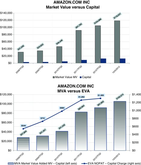
To give one example, consider Amazon, which produced the 38th highest shareholder return among the S&P 500 nonfinancials over the three years ending mid-2012. AMZN invested very aggressively in those years. Its capital surged from $3.4 billion to $13.0 billion, way outstripping internally generated sources. The spending was so intense that the Internet retailer’s cash flow net of the investment spending—the cash flow that you discount to measure value and that I refer to as its free cash flow—was negative $4.65 billion over a time frame when the firm’s stock price increased from $83.66 to $228.35 a share.
What explains why the stock performed so well while management was shoveling bucket loads of cash back into the business? The investments were paying off, and they were generating year-over-year increases in EVA. As is shown in Exhibit 2.4, AMZN’s EVA increased fairly steadily from $731 million for the four-quarter year ending mid-2009 to $1.3 billion for the mid-2012 year. As with Ball, AMZN’s EVA propelled MVA, which blossomed from $32 billion to $92 billion, for $60 billion of wealth created above all the capital infusions. AMZN illustrates a general rule: When cash flow goes down and EVA goes up, it’s EVA that wins the argument.
Exhibit 2.4 Amazon’s MVA and EVA (dollars in millions)
The implication is perhaps startling. You should stop using discounted cash flow analysis. That’s right. Stop using discounted cash flow. Cash flow is not wrong in principle. It does discount to NPV, after all, and NPV is still the goal. Cash flow just doesn’t work well in practice.
The only time management assembles all of the cash flow numbers in one view is when an investment is first proposed. But once accepted and funded, the capital is buried on the firm’s balance sheet and no one really seems to care too much about it. As a result, operating teams have a burning desire to get their hands on as much capital as possible, to build their businesses, pad their budgets, and grease the skids for bonuses and advancement. Knowing this, the CFO office deploys storm troopers to the field to check forecast assumptions. The field retaliates by raising the projections. The head office fires back with increases in the hurdle rates. And in the end, the whole process of capital budgeting is characterized by mutual deception and Kabuki theater—everyone is wearing a mask. And all of these shenanigans happen for a simple reason: because cash flow is being used to calculate the value of the plans and projects when cash flow cannot be used to measure their performance after the fact.
What’s better? EVA. Forecast, analyze, and discount EVA as the means to measure and improve the value of plans, projects, acquisitions, and decisions—as Volkswagen and Ball and many other EVA companies do—and then also measure EVA and reward improvements based on actual results. The NPV answer is always exactly the same. But unlike cash flow, EVA is able to forge a direct link between how decisions are made looking forward and how performance is measured and bonuses are awarded after the fact. It’s all EVA-based. And that consistency in both directions is the key to keeping it simple and keeping it accountable.
The logic of this recommendation won’t be fully apparent until I introduce the EVA performance ratios later on and show how they can be used to illuminate the moving parts that are driving EVA and driving the net present value. But the really important point for now is that, if you adopt the goal to increase EVA as the key profit performance measure, you are in fact motivating decisions that will maximize the discounted cash flow net present value of the business, and you can do that even better than using cash flow itself or any other financial measure.
VALUATION DETAILS
Establishing a connection from EVA to MVA and NPV, and to share price, is such a key consideration, and discarding cash flow in favor of EVA is so worthwhile, that it is worth going into more details on how this works. If you lack the patience for it, skip ahead. If you are on the quest, read on.
Let’s revive the simple sample company and value it using cash flow and EVA. Recall that SSCo is earning NOPAT of $150 and has invested $1,000 in capital. Let’s start with a simple example before layering on more realistic assumptions. We assume that the company will invest only to maintain its capital base and not for expanding it. It will spend only an amount equal to the depreciation of its physical assets and the amortization of its intangible ones, with two consequences.
First, its NOPAT profit will not grow. NOPAT will remain forever frozen at $150 because we are assuming there is no investment to grow the business; the only investment is to maintain it. Depreciation and amortization are deducted from NOPAT and equal amounts are invested to maintain the firm’s productive capacity and profit potential, but nothing more. This leads to the second consequence, which is that the firm’s capital is also constant. It runs at $1,000 forever. The maintenance capital-expenditure spending adds to capital each year, but that merely offsets the depreciation and amortization for the year, so that the net capital balance does not change.
The result is that the company’s free cash flow (FCF) is also frozen at $150. FCF is the net cash generated from operations after investment spending. It is the net cash available for investor distribution. And last, it is the cash flow that is discounted at the cost of capital to measure value.
The formula to compute FCF is to take the NOPAT earned on the income statement and to deduct the period-to-period change in the capital employed on the balance sheet. Since the net change in capital is zero in this case, the distributable free cash flow is simply the firm’s NOPAT profit. This reveals NOPAT’s true significance. It measures the after-tax operating profit that can be sustained indefinitely and distributed as a return to investors each year while preserving the integrity of the underlying capital base.
What is the value of the company under these circumstances? The company is like a bond that promises to pay $150 annually forever. The formula to compute the value of a forever payment is to divide it by the cost of capital. In this case, take the NOPAT of $150 and divide it by the cost of capital of 10 percent, and the company is worth $1,500. It is worth $1,500 because at that value, the $150 in NOPAT the firm earns and pays out each year always provides investors with the 10 percent return they are seeking.
Incidentally, the NOPAT that is capitalized to measure the value should represent the firm’s midcycle profit power, or the average NOPAT it will earn over a cycle. As a result, the return the investors earn on the market value they pay will actually fluctuate over business cycles, and won’t be an even 10 percent a year even if it is an average of 10 percent a year, which is why the expected NOPAT is discounted at the cost of capital risk rate and not at the risk-free government bond rate.
What is the firm’s MVA? The firm’s market value is $1,500 and its invested capital is $1,000. MVA is $500, the difference. The company has added $500 to the value of its invested capital. It has created a positive franchise value and has added to its owners’ wealth. This is depicted in Exhibit 2.5.
Exhibit 2.5 Market Value and MVA
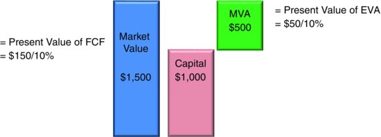
Now let’s use EVA to value the company with the same assumptions. EVA, recall, is $50. It is the $150 NOPAT less the $100 capital charge required to earn a 10 percent return on the $1,000 of invested capital. Since we’ve assumed NOPAT and capital remain the same forever, EVA will, too. It will run at $50 as far as the eye can see. The present value of earning $50 per year, discounted at the 10 percent cost of capital, is $500. Voilà, as advertised, the present value of EVA does indeed equal the value added to the capital. It discounts to NPV and MVA because EVA sets aside the profit that must be earned to recover the value of the capital.
Incidentally, the $500 MVA we just computed goes by another name. I call it CVA, for current value added. CVA is the MVA that comes from assuming EVA will hold steady at its current level and never grow or shrink, which is what we assumed in this special case. MVA can be greater than that, however, if investors expect that EVA will grow, which is the case we will now take up.
Let’s consider a more realistic example where the company invests capital and grows NOPAT and EVA. To keep it simple, assume that in addition to its normal replenishment spending to maintain the assets every year, the company makes a single growth investment of $100 in forecast year 1. Assume the payoff is that the NOPAT increases from $150 in year one to $165 in year 2 and then it holds steady thereafter (we’re assuming for simplicity that it takes a year from the time of the investment until the return kicks in).
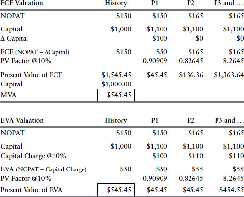
The company’s free cash flow (FCF) takes a major wallop in the first projection period. FCF drops from $150 to $50 as the $100 growth investment is deducted from NOPAT. Thereafter, assuming no more investment above maintenance spending, FCF continues forever at the new NOPAT of $165. Question: Is the company’s value higher or lower, assuming the forecast assumptions given are accurate? Cash flow per se does not help to answer that question. It is lower up front, and more later, so who knows? Cash flow provides an insight only when the stream of cash flow is discounted to a present value. So let’s do that, one last time.
As shown in the table, the FCF projected for years 1 and 2 is discounted to present value using conventional present value (PV) factors at the 10 percent cost of capital. The value of receiving $1 in year 1 is 90.90 cents today, and the value of a $1 in year 2 is 82.65 cents today. The trick is the PV factor for the third projected period, which is 8.2645. That says that each $1 of NOPAT that goes on forever starting in the third period is worth $8.2645 today. How so?
First, compute the value of receiving $1 of NOPAT per year forever at the 10 percent cost of capital. That is $1 divided by 10 percent, or $10. A 10:1 valuation multiple is put on each $1 of NOPAT. But that’s the valuation multiple as of the end of the second period, and we want the valuation now. We need to bring the valuation back two more periods to the present value. That’s easy. Just multiply the 10× multiple by the present value factor for the prior year, which recall is 0.82645, and sure enough, 10 times 0.82645 is the advertised 8.2645. That factor automatically computes the value of receiving $1 in NOPAT per year in perpetuity starting in period 3 and discounts it back two more years to present value. It is the present value of the enterprise multiple.
Multiply that factor times the projected perpetual NOPAT of $165, and the total present value is $1,363.64. Now add in the present values for FCF computed for the first two years, and the total present value of the cash to be cast off over the entire life of the business is $1,545.45, compared to a cash flow value of $1,500 before. The investment will bring an increase in net present value and MVA and increase the stock price. Just the prospect of the investment will increase the current wealth of the owners to a revised market-to-book spread of $545.45 versus $500 before.
That is all well and good, but why is that the answer? Why has the net present value increased? Cash flow tells us the value is higher but is silent on why. It swoons as the investment is made, surges as the return materializes, then flattens forever. What does the zigzag pattern tell us about the company’s performance and its value? Absolutely nothing. As I have said, cash flow gives an NPV answer but without any insight and without any accountability or line of sight back to how performance can be measured and rewarded. It is arid and isolated, and it must go. Let’s now take a look at how EVA values the same forecast, which appears in the bottom table.
As the $100 investment is added to the capital till, the capital charge increases by $10, from $100 to $110. That’s where the accountability comes into play. The cost of the added capital becomes a new and ongoing charge to the EVA earnings, and managers know they must beat that. In this case the increase in the capital charge is more than covered by the projected $15 increase in NOPAT. EVA is projected to increase by $5, from $50 to $55. The investment is EVA positive, and hence it is by definition NPV positive. The increase in EVA from $50 to $55 is a clear proxy for the added value. That is the insight that EVA offers that cash flow does not.
Using the exact same PV factors to discount the projected EVA as we used to discount cash flow, the present value sum is identical. The PV of EVA is the same $545.45 MVA that was derived from discounting the cash flow. NPV and owner wealth have increased from $500 to $545.45 because the present value of the stream of EVA has been projected to increase. EVA can do everything cash flow does as far as measuring NPV and value is concerned, but it also provides a period-by-period measure to explain why the value has increased or decreased. Outside a firm’s treasury department, which must be concerned with cash flow and how it will be financed and disposed of, there is no need for line teams to ever use it or be confused by it.
All other investments and returns are just variations on this simple example. It serves to show, I hope convincingly, that the present value of projected EVA always equals NPV at the investment project level and always equals MVA at the corporate level, no matter how complicated the pattern of investments and returns becomes.
Incidentally, there is a name for the added value we projected in this example. The extra $45.45 in MVA is called FVA, standing for future value added. It is present value of the growth in EVA over its current level. To put this in symbols, MVA = CVA + FVA. In this case, MVA = $545.45. That is the total NPV and wealth created. CVA = $500, and is the NPV value of the embedded EVA; FVA is the balance, $45.45, and is the NPV of the projected growth in EVA from $50 to $55.
In this example, FVA came entirely from the growth in EVA that was projected to occur in just a single period. In reality, FVA is the present value of the EVA growth that is expected over the entire life of a business. Does this require the clairvoyance of a Delphic oracle? Must EVA be forecast forever? Fortunately, no. EVA growth forecasts can be truncated as a practical matter. Here’s why.
Investors have learned from painful experience that competition, saturation, substitution, fading fads, bureaucratic creep, overpriced acquisitions, and outright management blunders are among the factors that eventually undermine a firm’s ability to continue growing its EVA. Like people, companies mature and lose their mojo. And when companies reach the point where their EVA can no longer grow, or are projected to reach that status, the EVA earned up to that point can be assumed to persist and be very simply valued in perpetuity. All business valuation methods do this, in effect. They reach a point where a terminal value is determined. But the justification for that lies in the EVA model and only in the EVA model. In all other models the rationalization for the terminal value is essentially a great mystery.
It is not just the saturation of the product and service markets that the company serves that sets limits on EVA growth. It is not that there is a given finite pool of economic profit to exploit, like a reservoir of oil to be tapped. The EVA reservoirs all have leaks. Emerging superior technologies and shifting tastes are always working to siphon EVA away underground and in an invisible way.
Think of it like this. When the world begins to value hot new things, the value it attaches to existing things cools, of necessity. Each consumer gets only so many votes to spend on the world market, and if consumers start to vote for the hot new things, like, for example, investments in social networking businesses, then they are implicitly withdrawing votes and subtracting economic profits from every other product and service and business out there. Think of EVA as the signal the market bestows on what it values and what deserves access to the available scarce resources for growth. Not everything can be a priority. As new businesses emerge and new technologies arise, the priorities change, the votes shift, and the EVA moves. Existing businesses wake up to find they have less pricing power and that they have become more like a commodity that can just cover its full costs, including the cost of capital, but no more. This can be frustrating. Management sees no reason for it. No bell goes off. But that is why it is so essential to monitor the movements of EVA at the margin.
Later on, in Chapter 7, Setting EVA Targets, we review statistics for the Russell 3000 companies over a 20-year history. You will see that EVA profits of individual companies definitely tend to cool and converge to long-run norms over time, and that the expectations factored into stock prices reflect that tendency. It is not just a theory.
Granted, some companies have managed to defy the gravitational pull on profits for a very long time. Coca-Cola is still increasing its EVA after well over a century in business, for example; but such companies are rare exceptions. Just think General Motors, Sears, Kodak, and RadioShack. Even once-revered tech giants like Hewlett-Packard, Dell, and Xerox have been just treading EVA water in recent years. Their EVAs are moving sideways as their products become more perfunctory. Their EVA glory runs appear to be at an end unless management can pull off a miraculous revival. Hope springs eternal, and some may succeed. But when real money is on the line, investors almost always assume that a company’s EVA will eventually crest, and they will not take the risk of assuming it will grow forever.
This is the hard part of the valuation business. How long do you forecast it will take before Wal-Mart exhausts its profitable growth opportunities and its EVA no longer grows, for example? Are Best Buy and Dell already at the end of their EVA growth curves, or will they revive? And perhaps the biggest question of all: How long before Apple becomes like Whirlpool, a maker of everyday appliances in a crowded competitive market where increasing EVA is really hard to do?
Bear in mind that we are talking about growth in EVA and when that stops. Companies may continue to expand for quite a while, open new stores, add new customers, develop new products, increase sales and earnings, and so on, and yet see their EVA go sideways as they just earn the cost of capital on net on all new investments. This is far from a question of forecasting when a bankruptcy will occur. It is a question of when a sector becomes so competitive that the prices companies can charge will just cover the total cost of all resources they use. At that point there is no incentive for a new entrant to jump in and make matters worse, but neither is there an incentive for investors to pay a premium for growth even though the growth in sales and earnings per share (EPS) may continue for quite a while. All other measures are blissfully ignorant of the competitive change that has made growth irrelevant to the valuation of the company. But not EVA.
Please understand that EVA does not make valuations harder by asking these questions. Quite the opposite. EVA helps make valuations easier and more accurate by bringing the question of when growth will no longer add value and when EVA will crest into sharp relief. Other models simply ignore the issue or obscurely bury it in indeterminate valuation multiples.
Let’s probe the question a little further. The EVA growth horizon that investors forecast typically involves some judgment about a particular company, but with heavy overtones from a probabilistic and pooled estimate. Stocks, in other words, are priced a lot like life insurance policies. No one can predict when any one person will expire, but the pool is predictable. You can look it up in actuarial tables. The same is true of stocks. Firms of a certain character, ones for example that have long-established profitable franchises and economic moats that protect them from encroachment, are as a group assumed to live longer EVA lives. They are the nonsmokers in the valuation crowd with healthy DNA. Some of the firms in the pool may sustain EVA growth for longer than the median estimate, others less, but the market will tend to get the pool right on average. And for well-endowed firms like these, the market generally prices seven to 12 years of EVA growth into the stock, but those estimates are revised all the time.
On the other side are firms in highly competitive businesses with many rivals and with little lasting opportunity for differentiation. Think of airlines or grocery chains, for instance. The firms are for the most part run by intelligent, dedicated, and creative people, but it is very easy for competitors to imitate what works. There are exceptions like Alaska Air and Whole Foods—that is where the company overlay comes in—but in the main, the market will not embed any significant expected EVA growth into the MVA of these stocks at any time.
The next category covers firms whose EVA profits are purely cyclical or commodity-price-driven phenomena, like fertilizer or forest products companies. From experience, the market assumes that any windfall or shortfall in the EVA profits is temporary and will be swiftly competed away or reversed as a normal supply/demand balance is restored. But putting the cycles aside, the EVA growth horizon for those firms is really nearly always zero.
In between the EVA-endowed franchises and the EVA-lean cyclical or commodity firms are two other categories. The first I call the flashes in a pan—companies that get hot and ride a wave and produce impressive EVA profits for a while, but are highly vulnerable—think Research In Motion (BlackBerry) or Nokia or Motorola in the cell phone business, or Green Mountain Coffee with its Keurig machines (now that Starbucks is on its tail). Their EVA can disappear in a blink of an eye and often does. The market always fears that will happen and factors the possibility into an actuarially limited EVA growth horizon, which is one reason why the managers in those firms are always dissatisfied with their market valuations.
The last category of note are the middle-of-the-roaders, the everyday firms operating in businesses that still have modest to above-average growth prospects, and where technological or brand or organizational capabilities confer the ability to sustain EVA growth over some reasonable horizon. How long? The general rule is five years. For most companies, the market is willing to pay for about five years of growth in EVA, and then assumes, either literally or effectively, that EVA flattens there forever (EVA may actually be forecast to continue growing for a while longer but then to fade, with the same valuation effect as if it was level forever). Even if you can sit down with your computer and forecast 50 years (Excel is a wonderful extrapolation tool), the market is apt to pay for only five, except in special cases. It is particularly important to recognize this limitation when you are pricing an acquisition candidate. It is easy to overpay by assuming EVA will grow for a longer stretch than the market will ever pay for.
Now let’s return to the conversation about FVA—the portion of the value that is due to growth in EVA. It can be derived from discounting a projection of EVA, taking account of the appropriate growth horizons per the earlier discussion. That is what we did in the simple valuation example we just covered. But there is also a way to derive FVA from share prices to see what the market thinks it is. To do that, we compute MVA from the company’s share price and then deduct its CVA—the MVA portion determined by capitalizing the firm’s most recent four-quarter EVA at its cost of capital. The remainder is the firm’s implied FVA, and it measures the total present value of the growth in EVA that investors are implicitly forecasting. This calculation is a way to free ride on the research that investors have done and have registered in stock price bets. It won’t always be right, of course, but it is always worth consulting.
To illustrate, let’s take a look at Apple. Its EVA and MVA are portrayed in Exhibit 2.6 with a breakout of MVA into the CVA and FVA components. No surprises here—Apple has been a prodigious producer of EVA and MVA, the most prodigious ever. As shown in the lower left chart, Apple’s EVA—the line—was running at a sizable loss as recently as 2003, just nine years ago. But since then it accelerated to, gulp, over $28 billion for the four-quarter period ending in June 2012. That’s Apple’s EVA profit, not its sales, ladies and gentlemen. And whereas 15 years ago, in 1997, Apple’s MVA—the bar on the lower left chart— was negative, as of late summer 2012 it stood at, phew, $524 billion of created wealth and counting. As expected, Apple’s MVA increased in lockstep with its EVA.
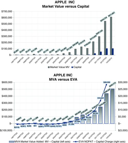
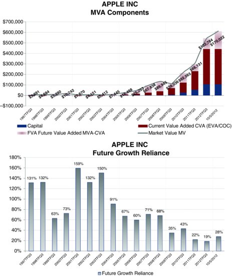
The upper left chart plots Apple’s aggregate market value as the light bar. The dark bar is the firm’s capital. The visual gap between them is MVA. Now look at the upper right chart. The line is aggregate market value once again, but now the bar below it has been divided into three segments, with capital at the bottom and a CVA component, which is the capitalized value of the EVA that Apple earned over the trailing four quarters, in the middle. The top portion of the bar is a plug residual component, FVA, which is the present value of the growth in EVA that investors are forecasting the firm will earn. That, too, increased from under $10 billion as little as eight years ago to $170 billion as of early October 2012.
Apple has not only performed magnificently. Steve Jobs and his successors brilliantly positioned the company to generate ever larger pools of EVA profit down the pike—or at least that is what the market is expecting. And that illustrates a general rule. Wealth creation and shareholder returns can generally come from just two sources. One is from actual performance, from raising the EVA performance bar and generating a greater CVA value. The second is from convincing the market that EVA will grow even faster than previously thought, which will translate into an increase in FVA. We will see this more formally a little later when we use EVA to explain shareholder returns.
The lower right chart in Exhibit 2.6 displays the ratio of FVA to market value, which I call Future Growth Reliance (FGR). It is the percentage of the firm’s market value that is implicitly counting on—and is at the risk of not getting—continued growth in EVA. As of early October 2012, 25 percent of Apple’s market value was banked on projected EVA growth. In the early years, when EVA was negative, as much as 160 percent of the company’s market value was premised on EVA growth. That was an indication of just how risky the stock really was at that time and how much, even then, the market was willing to gamble on Jobs pulling off a miracle.
As time passed, Jobs and his team worked their magic, and the forecast EVA materialized (actually, a whole lot more materialized than the market had forecast); a larger proportion of Apple’s market value shifted from potential value into actual value, from FVA into CVA, into the value of the embedded and established EVA profit stream and away from the expected growth. Don’t misunderstand this. A massive expectation for growth in EVA profits remains in the share price, but the percentage of the firm’s market value that is represented by that and is premised on achieving further EVA growth has shrunk.
To conclude, then, Future Growth Reliance (FGR) is a ratio statistic that EVA Dimensions tracks and that CFOs and board members should monitor. It provides a convenient and reliable indication of the market’s confidence in a company’s turnaround plan or strategic positioning to grow EVA. Later on, we will take this a step further and show how to convert FGR into an even more usable statistic, which is the expected growth rate for EVA.
GETTING FROM EVA TO THE SHARE PRICE
At this point I am quite hopeful that you understand that projections of EVA can be used to model the NPV of capital projects and specific decisions, and that a consolidated EVA projection discounts to the corporate aggregate MVA. That still leaves the question of how to get from MVA to share price.
It’s easy. A little fiddling with the MVA formula is all that’s required. Recall that MVA is market value less capital, where capital is the net assets used in the business:
MVA = Market Value − Capital
Rearrange, and substitute for MVA:
Market Value = Capital + MVA
Market Value = Capital + Present value of EVA
In other words, the market value of a company as a going concern business is equal to the book value of the capital that has been put into the business plus a premium, or less a discount, to reflect the quality of capital management. Said another way, corporate market value is commodity capital value plus proprietary franchise value, where franchise value is measured by the present value of the projected economic profit. For example, the market value of Microsoft is the money spent developing the software code as if it were just random zeros and ones plus the franchise value of the code in the sense that it works and it enhances the productivity of Microsoft’s customers.
The franchise value could come from technology and innovation, distinctive and trusted brands, exceptional customer service and satisfaction, operational excellence, or any of myriad operating or strategic elements that enable the company to charge a price in excess of the total resource cost and to earn a positive EVA profit. If an asset does not ever appear in EVA, then it is not a real asset. A brand, for instance, has value only if it can be, and at some point is, used to create EVA.
So to determine a company’s share price, follow these steps:
Don’t get lost in the recipe. Follow it through and you realize that since most of the factors don’t change, at any point in time the stock price is essentially just a function of adding the projected MVA per share to the common book value per share (as adjusted for accounting distortions we’ll get to in the next chapter). If a company has 100 common shares outstanding, a corrected common book value of $1,000 (i.e., $10 a share), and a projected MVA from discounting EVA of $500 (i.e., $5 per share), then the stock has an intrinsic value of $15 per share, the sum. And since the book value is set at any instant, the only way a company’s stock price increases is if management can earn more EVA and credibly increase expectations for earning even more EVA, as I demonstrated with Apple and will quantify further in the next section.
Once you have gone from EVA to share price in the four-step process I’ve laid out, you may want to compute various multiples to see how the valuation stacks up with other companies. You may compute a price-to-book or price-to-earnings multiple, or an enterprise valuation multiple that divides total value by the firm’s EBITDA, for instance. Fine, do that, and see how it stacks up. But don’t confuse cause with consequence.
To take the prior example, if the firm’s earnings per share are $1, and the stock is worth $15 based on discounting EVA, then the stock trades for 15 times earnings. Follow the words closely. I said it correctly. The stock is not worth $15 because it is worth 15 times earnings. It is worth 15 times earnings because EVA says the stock is worth $15. Accountants compute EPS. Price is determined by discounting EVA. The P/E multiple is just a plug—it’s the arithmetic relationship between the earnings that accountants calculate and the share price that EVA determines. It is the result of the valuation, not the source of it.
Many CFOs get this backward and confuse cause with consequence. They assume their stock price is a result of the multiple. They will say, “Our stock trades for $15 because we trade for 15 times earnings.” That’s completely ass backwards. The word because is fatal; if you believe stock prices result from the market applying a multiple, then you believe the best way to increase your stock price is to increase the denominator of whatever multiple you like the most. And if you do that, odds are you will end up killing your EVA and your stock price.
If you cotton to P/E, you aim to increase the E, the earnings per share, and you move mountains to avoid diluting EPS. If enterprise multiple is what you fancy, then you go on a warpath for more EBITDA. You are willing to spend any amount on capital so long as you improve cash profit. And if price-to-book is your cup of tea, you grow the book value. You retain earnings and add assets that increase your capital charge and reduce your EVA. In each case, you are literally aiming at measures that will almost guarantee you will kill your firm’s EVA and end up trading for a much lower multiple of whatever denominator measure you used as your performance goal.
THE TIE BETWEEN EVA AND SHAREHOLDER RETURNS
I’ve always thought it was obvious and uncontestable that the corporate mission is to maximize owner wealth—to allocate, manage, and deploy resources to maximize NPV, which at the corporate level is manifest in MVA. After all, the title of Adam Smith’s book is The Wealth of Nations, not the returns of nations. Creating wealth is the name of the game, and has been from the beginning. And I always felt that if a manager took care of maximizing wealth, then the returns that the shareholders earned would be maximized, too, as a natural by-product and not as something separate and distinct to worry about.
Many CFOs are not satisfied with that answer, though. They are stuck on explaining shareholder returns, even though maximizing wealth and increasing MVA are the better goal. But the CFO is my client, so I decided one day to derive the exact link between EVA and shareholder returns. I burned out my pencil sharpener but finally got it. For those who can’t sleep at night without knowing the answer, read on. All others can take my word for it and safely slip into the next chapter.
Let’s start with the axiomatic assertion that shareholder returns are defined as the dividends shareholders receive plus the appreciation in value of their shares, divided by the share price at the beginning of the measurement period. The total shareholder return (TSR), in other words, is a function of cash yield and a cash-equivalent gain or loss. It’s a cash-on-cash return, in effect. That is by definition.
EVA does not tie directly to TSR, but we can get there eventually. EVA actually ties to a broader definition of return, what I call the total investor return (TIR). It is the return the company generates on behalf of all investors—its lenders and shareholders combined. In other words, it is the return on the total enterprise value of the business. It’s the return you’d get if you bought the stock and the bonds and held all of the liabilities of the company (except trade credit) in market value proportions.
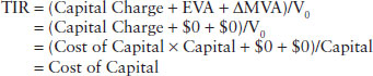
Like TSR, TIR can be estimated from a cash-on-cash yield. It is the free cash flow (FCF) the business generates, plus the change in the firm’s overall market value (ΔV), divided by its market value at the start of the period (V0), again, by definition.1 I write it like this: TIR = (FCF + ΔV)/V0.
Now let’s play the substitution game. We know FCF is NOPAT less the change in capital (i.e., FCF = NOPAT − ΔCapital). Since EVA = NOPAT − Capital charge, then NOPAT = Capital charge + EVA, so plug in:
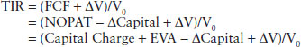
And because MVA = V − Capital, and thus ΔMVA = ΔV − ΔCapital, TIR reduces to:

The revised formula shows that the total return a firm generates for all investors is a function of three factors that all come from the EVA model. The first factor is the capital charge/beginning value. It comes from simply reversing the discounting process. As time passes, investors earn a return from the time value of the money. The charge for using capital that is built into EVA is in fact the basic source of the return to investors, which is why acknowledging and earning the charge is so essential to good corporate governance.
The second factor comes from earning EVA. The more EVA, the higher the return. It’s one for one.
The third factor is the return that comes from increasing MVA. As I have already established, MVA increases when the expected present value stream of EVA increases from improvements in either CVA or FVA, or both. In other words, the true drivers of shareholder returns, beyond just passively reversing the discounting process, are earning and increasing EVA and increasing expectations for earning even more EVA. True, the returns are paid in the currency of cash and cash-equivalent value change. But don’t be deceived—the cash is just the medium of exchange. The actual driver of shareholder return is (no surprise here) EVA all the way!
Let’s put the simple formula through its paces. Suppose a company is just breaking even on EVA and is not expected to improve it. In that case, it trades at the value of its book capital. Its MVA is zero and is not expected to increase, because its EVA is zero and not expected to increase. TIR is reduced to just the capital charge yield on the value:
Since market value equals the capital in this case, the charge for capital delivers a cost-of-capital return on the value. TIR equals the cost of capital, every year, as expected.
Now suppose the company belches out a one-time unexpected EVA uptick that has no impact on expected future EVA and so none on MVA or market value as well. Then the investor return that year will increase by the one-time EVA uptick, but no more, and thereafter it will settle right back to the cost of capital. Nonrecurring profits pay a one-time bonus dividend but just don’t move the market. There’s an important message there. Managers should avoid spending a lot of time on generating one-time gains since the market will assign them a multiple of one, then none.
Now suppose the firm’s EVA rises and investors consider the improvement permanent. The firm’s MVA increases to incorporate the increase in projected EVA, and the investor return soars whenever investors are first convinced this will happen. Depending on the cost of capital, the MVA increase could be 7 to 20 times the increase in annual EVA.
Finally, suppose that investors not only expect the increase in EVA to be permanent, but they also believe that management has positioned the company to continue increasing EVA for some time. In this case, MVA is turbocharged as both CVA and FVA rev up. The investor return skyrockets when the long-run EVA trajectory is revised and impounded into the share price. That, of course, is exactly what happened to Apple. EVA increased prodigiously, and the market now projects it to continue growing for quite a while. But that was not the case at all 10 years back.
After such a run-up, TIR will be based off a much higher market value. To just earn the expected cost of capital, a company like Apple will need to continue to increase its EVA and hike up its MVA year over year just to stay on track with expectations. But that is the way markets work. And it is another reason why I think it is helpful to have incentive plans that reward managers not only for increasing the stock price but also for actually delivering the EVA profit growth the market is expecting.
Recall that TIR measures the return earned on behalf of all capital providers, including lenders, whereas TSR is the return just for the common share owners. It is easy to go from one to the other. TSR is simply a leveraged version of TIR. The formula is:
TSR = TIR + (TIR − BR) × (D/E)
It says that TIR is first applied to pay interest expense and other prior claim returns (as represented by BR, standing for the overall average borrowing rate paid to senior claimants), and what’s left over is then spread over the common equity portion of the market value, so the higher the firm’s debt-to-equity (D/E) ratio, the more any TIR excess return is magnified, up or down, for good or ill, into the shareholder return.
For instance, suppose TIR is 26 percent, the average effective borrowing rate is 6 percent, and the D/E ratio is 50 percent. Then the TSR that year would be 36 percent.
TSR = 26% + (26% − 6%) × 50% = 36%
Leverage cuts both ways. If TIR is −14 percent, then the firm’s TSR would be −24 percent.
TSR = −14% + (−14% − 6%) × 50% = −24%
The bottom line is that total shareholder return is still very directly a function of EVA and any changes in expectations for EVA, only with leverage thrown in to spice it up.
Let’s test that proposition with an application to Ecolab, currently with about $7 billion in revenues from cleaning and sanitizing chemicals following its acquisition of Nalco. Exhibit 2.7 displays the total investor return computed each year from the capital charge, EVA, and change in MVA over the year, divided by the initial market value, and the total shareholder return computed the conventional way from dividends and capital gains on prior share price. The light dashed line is the ratio of market value to equity value, so, the larger it is, the more leveraged the firm was.
Exhibit 2.7 Ecolab’s Total Shareholder Return and Total Investor Return
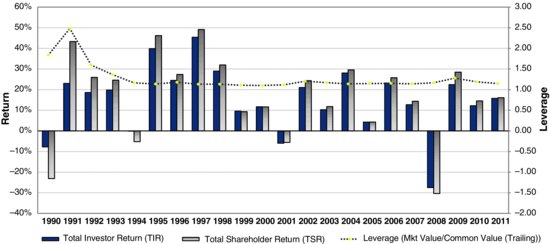
What is striking is how similar the two returns are, even though they are computed from two entirely different formulas. TIR is computed strictly from the EVA metrics related to the firm’s overall market value, TSR from cash dividends and cash-equivalent capital gains on the share price. Yet, the two were extremely highly correlated for Ecolab. In other words, the math derivation works! And not just for Ecolab. If you run the correlation across all stocks, it is about 82 percent. Maximize EVA, maximize MVA, and the shareholder returns take care of themselves. I’ve said that for many years, without any mathematical proof, but now there it is. It must work as long as 2 + 2 = 4.
The only notable exceptions to this rule for Ecolab were in the early 1990s because Ecolab was highly leveraged at the time. Back then, market value was around 2 times equity value, or, put another way, debt was 50 percent of market value. A surge in TIR in 1991 and a downdraft the year before were strongly amplified in TSR. But that’s just noise and should not distract from the essential conclusion. EVA is, in principle and in practice, the true driver of shareholder returns. No other measure can make that claim.
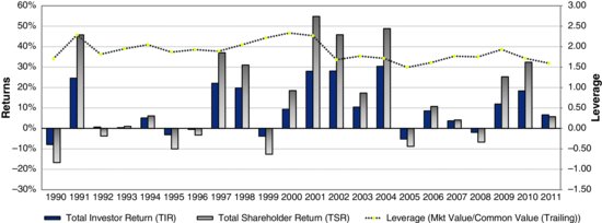
The same chart for Ball appears in Exhibit 2.8. The correlation between the up and down movements in the total EVA return on value and the total shareholder return is again very high, as expected. It is still EVA that is driving the returns. But the two return series are not as close in each period as they were for Ecolab because Ball has typically employed a lot more leverage. Keeping debt leverage high is one way that Ball’s management has kept its overall cost of capital low to help keep its EVA high. And, in this case, the leverage has amplified mostly positive investor returns into even higher shareholder returns, which has been a blessing. If a management team is really confident about earning EVA, why share it? Use more debt and less equity to lavish the excess returns on the investors who get the EVA story.
Exhibit 2.8 Ball Corporation’s Total Shareholder Return and Total Investor Return
1 In practice it gets a little more complicated when we consider excess cash holdings that are excluded from the definition of FCF but that can also be paid out or accumulated in a period, or if a company spins off a major line of business, and so on. But those are details that do not alter the insights I will explain.