CHAPTER 3

__________________________

EMPLOYING FUNCTIONS

Perhaps one of the most fundamental concepts in engineering (and mathematics in general) is the idea of a function. Without this brilliant mathematical object, the remainder of this text and engineering-based mathematics beyond these pages would likely not exist! (At least not in the same form.)

 

3.1 RELATIONS TO FUNCTIONS

Informally, a function is rule that takes inputs and assigns a value to them, an output. Functions are frequently denoted by f(x), where the name of the function is f and the input is x. Take care to note the difference between a system and a function; the analogy is almost identical, but functions will be primarily used to characterize the inputs and outputs of systems.

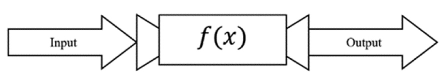
Functions are based on the simple premise of a machine that receives an input and sends something out (an output). This machine is commonly called f(x) (Figure 3.1).

 

Figure 3.1. Visualizing a function

Each input produces a unique output; this means that any input cannot result in two or more different answers. If the function machine takes the input “2” and assigns “0” and “1” as outputs, the machine is broken...and we do not have a function. Our complete definition is as follows.

Definition 3.1: A function is a relation that uniquely assigns elements of one set of inputs to elements of a set of outputs.

The term relation has a technical meaning, but all we will do is drop one important word from the definition of a function—“uniquely.”

Definition 3.2: A relation assigns elements of one set of inputs to elements of a set of outputs.

What’s the difference? We have two sets of data that are related through some process in both situations—which automatically fits the definition of a relation. If each input has a unique output, then it can also be called a function. Figure 3.2 demonstrates a situation where f (x) is not a function.

 

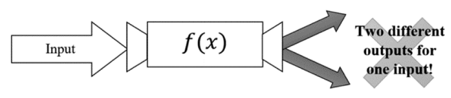
Figure 3.2. When f (x) is NOT a function—one input yielding two (or more) different answers

On the other hand, different inputs can have the same outputs—we would still have a function (Figure 3.3).

 

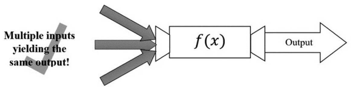
Figure 3.3. Multiple inputs yielding the same output still means f(x) is a function

Examining these definitions shows that every function is also a relation (there is a relationship between the input and output), but not every relation is a function. We can give the collections of inputs and outputs more specific names: The set of all of the inputs that we can plug into the function is called the domain, whereas the values that are coming out, the outputs, are collectively known as the range.

Definition 3.3: The domain is the set of values for which a function is defined.

Definition 3.4: The range is the set of possible values resulting from plugging the values from the domain into the function.

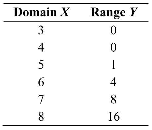
Example 3.1: Determining Functions—One method of defining a function is to list the possible inputs (the domain) and corresponding outputs (the range) as shown in Table 3.1. When creating a column to write inputs and outputs, the x column is the domain, whereas the y column is the range.

Table 3.1. Domain and range of a simple function

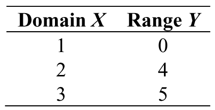
We can determine what is and what is not a function in a few different ways. One method is simply checking each pair in the table. Is Table 3.1 a function? Remember that each input must only produce one output (in our example, when we input 2, it produces 4—period—it never yields a different number). Through inspection, our example above passes the test because each input has its own output. What about Table 3.2?

Table 3.2. A function with more inputs and outputs

Instead of looking at Table 3.2 as a standard list of values, we could write each x value down in one column, each possible y value in another column (do not repeat outputs if they occur more than once), and connect each input to an output with arrows (Figure 3.4).

 

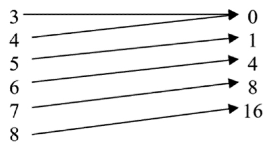
Figure 3.4. Drawing out the function using arrows

The function in Figure 3.4 also passes our requirements to be a function. Do not let the repeated zero be of any concern; if two inputs have the same output, there is nothing to worry about. We will look at one more relation as shown in Table 3.3.

Table 3.3. One last possible function

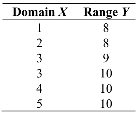
Rearranged into a mapping in Figure 3.5...

 

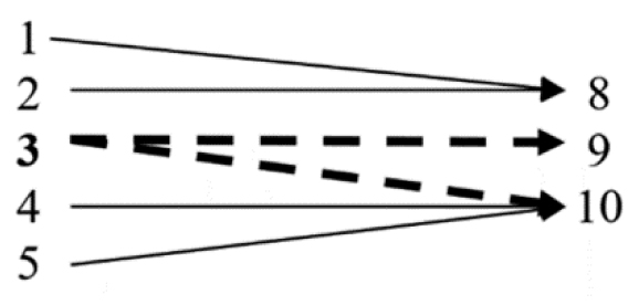
Figure 3.5. Realizing the mapping is not a function

Figure 3.5 is a bit different than the previous two functions; we have five inputs and three different outputs. This would be alright, but if we plug 3 into the function, we obtain 9 and 10—this is not allowed based on our definition. Therefore, Table 3.3 (and consequently, Figure 3.5) is not a function, but it is still a relation.

***

We used function notation earlier when we were naming our machine by writing f(x). With this notation, we are naming our function f and then claiming the variable is x. Now that inputs and outputs of functions are established, we can start using the common notation with these ideas in a more concrete fashion. For functions, x is the input variable: x can represent any value within the domain. The variable does not have to be x; it could be t, a, β, or any symbol we choose—x is just the name of the variable. Whatever values are in the domain of f can replace x in the parentheses of f(x). For example, if we plug 1 into f(x), then we would write f(1). Then, f(1) would correspond to some value within the range of the function. To translate the full statement into function notation, “plugging 1 into f(x) results in 0,” would be the same as writing “f (1) = 0” (Figure 3.6).

 

Figure 3.6. Function f with input of 1 gives an output of 0

Example 3.2: Evaluating a Function at Different Points—Let us evaluate the function f(x) = x² – 1 at the points x = 1 and x = 2. For x = 1, all we need to do is replace x with 1 wherever x appears.

Therefore, f(1) = 0. At x = 2, we perform the exact same procedure:

This means f(2) = 3.

***

We already mentioned the concept of a domain, but figuring out which values are allowable is an issue now that our functions have precisely defined rules. Only certain values of x will be allowable in many cases, but the possible values are easily found.

Example 3.3: Finding the Domain and Range—Consider the function . Think about the numbers x could be and how its value would affect f (x). We can quickly spot a square root sign—which means trouble. If the sign of the number under the radical turns out to be negative, then the result will not be real—think about the value of as an example. To compensate, we need to find the set of allowable inputs by making sure the inside of the radical (9 x²) is bigger or equal to zero. Therefore, we can form an inequality by, say, literally translating our intuition into symbols:

Then we can solve for x:

Taking the square root of both sides forces us to refine our inequality like so:

Therefore, our domain is D:[–3,3]—all real numbers between –3 and 3 including the end points. If we look into the domain, we notice that there will be a limited number of outputs. By plotting the function on a calculator or computer, we obtain a graph as shown in Figure 3.7. The highest point is at x = 0, meaning we can deduce f(0) = 3—this is the biggest number in the range. Since we cannot have negatives under the radical, it will be impossible to have negative numbers as a result. With the previous fact in mind, the smallest number in the range has to be zero; therefore, the range R is [0,3].

 

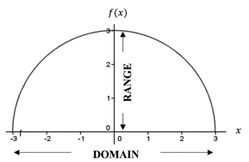
Figure 3.7. Domain and range of

 

3.1.1 COMPOSITION

Functions can be combined through an operation called composition.

Definition 3.5: Given two functions, the operation of composition, given by ∘, is performed by applying one function to the results of another.

Suppose we have two functions, f (x) and g(x), then we can use the symbol ∘ to denote composition, f∘g, (read as “f composed with g.”) In engineering, the open dot is replaced with different notation, f(g(x), which is read the same way. We can interpret the composition operation as a form of embedding information. For instance, the two pictures on the left in Figure 3.8 are separate; however, we can compose them to create the new image on the right. The leftmost picture is used as a template to guide the placement of the smaller picture, the smiley face. In terms of our functions, we can call the original picture on the left f and the additional detail on the right g. With our choices, the combined picture on the right is f(g(x)); since f is physically composed of g, the meaning of f(g(x) is quite literal.

 

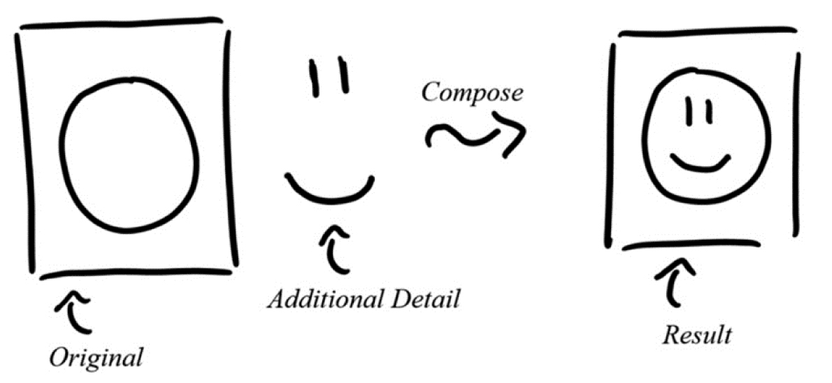
Figure 3.8. Embedding information into a picture

To illustrate with two functions, say f(x) = 1 + x + x² and g(x) = sin(x). If we compose f with g, then

Composition works like evaluating a function at a particular number; however, we are plugging in the entire g(x) function instead of a single number. If we swap the order of composition, the result looks completely different:

Looking at both compositions, it is safe to say f(g(x)) is not the same as g(f(x)—try by testing out different inputs like x = 0.

Within the context of engineering, we often use functional composition to embed information in terms of time, temperature, position, and so on.

Example 3.4: Composition of Functions to Embed Information—Harnessing the power of the wind is a popular form of alternative energy. Wind turbines are implemented to capture the kinetic energy of the wind and translate mechanical power to electrical power; however, turbines will not generate any usable power until the wind reaches a certain speed, the cut-in velocity. Although the turbine can generate power once the cut-in velocity is reached, the rated power—the maximum it can produce—is achieved at the nominal velocity of wind. Hurricane force winds will likely render the blades unusable, so there is a maximum wind speed where the turbine will cease producing power, the cut-out velocity. The output power of the turbine is dependent on the wind speed, meaning the power will be a function of wind speed, w; therefore, the base function is P(w). Wind speeds are bound to vary during the day, so we can loosely describe the wind speeds over the course of the day as a function of time w(t)—where time is in hours.

If we compose P with w(t), we will have a function describing the power produced by the turbine at any time during the day, P(w(t). With that simple step, composition encoded a bit of additional information into our function. Now we can easily see that the power depends on time in addition to the wind speed at that time.

Suppose our P function is given by

The w(t) function that tells us the wind speed for any time t will likely look more sophisticated in practice, but let us assume the wind is relatively constant throughout the day for the sake of simplicity (Figure 3.9).

If we compose P with w(t), then we will have

All we did was replace any w in the original P function by the new function, w(t). Now, if we want the power produced by the turbine at noon, then we would check the value of w(t) at t = 12 hours, w(12). Therefore, the power is

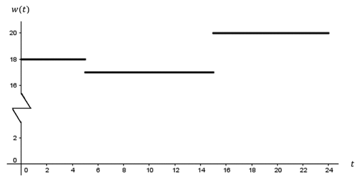
Figure 3.9. Plot of w(t)

In this case, the wind speed at noon is 17 meters per second—so w(12) = 17.

Note the change on the SI prefix because 110(17)³ [kilowatts] = 540430 [kilowatts]. We can simplify by noting “kilo-” means 10³ and 540430 can be written as 540.43 × 10³; therefore, the result is 540.43 x 10⁶ watts or 540.43 megawatts.

***

Example 3.5: Another Application—Electromagnetics—When we move a conductor—a material that lets electric current flow freely—through a magnetic field, then we can generate a voltage called motional electromotive force (emf). Let us say we have a metal bar and we drag it along metal rails, nothing special is going to happen besides a bit of clanging; however, we can generate a current if we happen to do this in the presence of a magnetic field (Figure 3.10). To find the motional emf due to moving the rod, we need to know the strength of the magnetic field B, the length of the rod l, and the velocity at which we move the rod u (this will be our variable).

Say we move the rod back and forth with the following function describing the velocity,

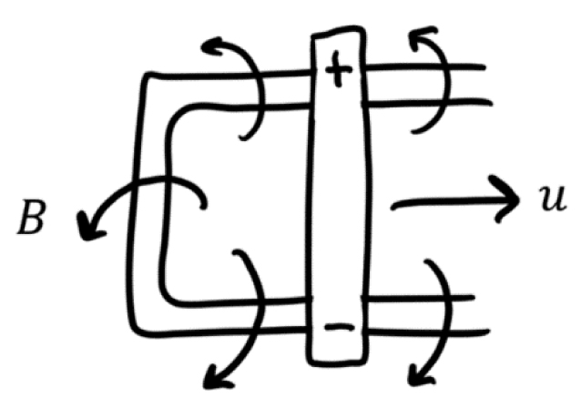
Figure 3.10. Sliding a metal rod along metal rails in the presence of a magnetic field

Like before, we can write the motional emf in terms of the time rather than velocity by forming the composition of V with u.

***

 

3.1.2 INVERSE FUNCTIONS

Imagine we’re typing out a five-page paper—an absolute masterpiece of an assignment, the perfect résumé, a well-crafted short story... Right as we are about to change the font to add a visual flair to the work, we accidently delete the entire thing...all of the progress completely disappears. No need to worry, we have the power to bring everything back with the “Undo” option in word processing applications. Now it is like we never deleted anything (Figure 3.11)!

 

Figure 3.11. Intuitive behavior of an inverse function

In mathematics, there does exist an “undo” button that we like to call an inverse function.

Definition 3.6: Given a function f (x), the inverse function is a function that undoes the action of f (x).

In the context of functions, the inverse undoes anything that the original function did. When we write the inverse symbolically, we usually denote it by f^–1(x). Note: we must completely disregard the instinct to say f^–1(x) = 1/f(x), the –1 is not an exponent.

Example 3.6: Finding the Inverse of a Function—Suppose we have a function, f(t) = 10t/(t + 3) describing the amount of water in a tank (measured in gallons) and we want to find a function g(A), which tells us the associated time for any amount of water, A. In this scenario, f(t) tells us how much water is in the tank at any time; for instance, if we plug in t = 2seconds,

we find the amount of water in the tank is 4 gallons. In words, the question the function f answered was, “How much water is in the tank at 2 seconds?” In terms of functions, we took a value from the domain of the function (t = 2) and found its associated value in the range (4). When finding the inverse, we are starting with the 4-gallon figure and asking ourselves: “At what time does the tank contain 4 gallons?” Our question places us the range instead (at A = 4), and we need to travel back to the domain if we want to find the value of t mapping to 4.

To find the inverse, we will start with what we know: At any time t, we can find the amount of water A in the tank—written as f(t) = A. Our function can then be rewritten as

Since we want the inverse of the function, we need an expression of the form t = something in terms of A. To achieve this, we need to solve for t. We can begin by multiplying both sides by t + 3 and distributing the A on the left-hand side.

Now we subtract At from both sides and factor out the t.

Finally, we divide both sides by (10–A) to arrive at the inverse function, f^–1.

Notice how the new expression is completely in terms of A, the water level. Now, for any amount of water A, we can find the associated time t—written as g(A) = t. Therefore,

If we plug in the 4 gallons we found earlier, our result should be the 2-second figure we were testing.

Since we found the inverse correctly, our work checks out!

***

The inverse function possesses a few notable properties, one of which provides us with a convenient way to check whether or not we found the correct inverse. For a function f and its inverse f^–1, then

In other words, if we compose a function with its inverse or vice versa, then the result will always be the input, x. As a consequence, the graph of f^–1 is obtained by mirroring the graph of f over the line y = x. To illustrate, consider f(x) = 2x and its inverse f^–1 (x) = x/2 in Figure 3.12. The mirror effect is easily seen, especially because f is linear in the example.

When we started talking about inverses, we informally thought of f^–1 as a mathematical undo button. To see why we chose to do so, watch what happens when we compose the two functions f(x) = 2x and f^–1 (x) = x/2 as f(f^–1(x)).

Figure 3.12. Graphical relationship between f and f^–1

Notice how the 2s canceled out? The original function involved multiplication while the inverse involved division—complete opposites in terms of arithmetic. If we compose the other way, we notice the exact same process happens:

This property holds for any function and its inverse—if correctly defined. The functions from our example were simple and linear, but if we play around with a few complicated functions, we tend to run into problems. To be more specific, the issue we need to discuss is lurking in the function’s domain.

Example 3.7: Restricting the Domain—To demonstrate the problem, let us take one of the simplest functions we can come up with, f(x) = x², and find its inverse. After using the procedure in Example 3.6, we quickly find the inverse, 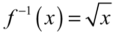. Yet, if we look at the graphs of f(x) and f^–1(x) in the same plot (Figure 3.13), it appears as though the mirroring property failed.

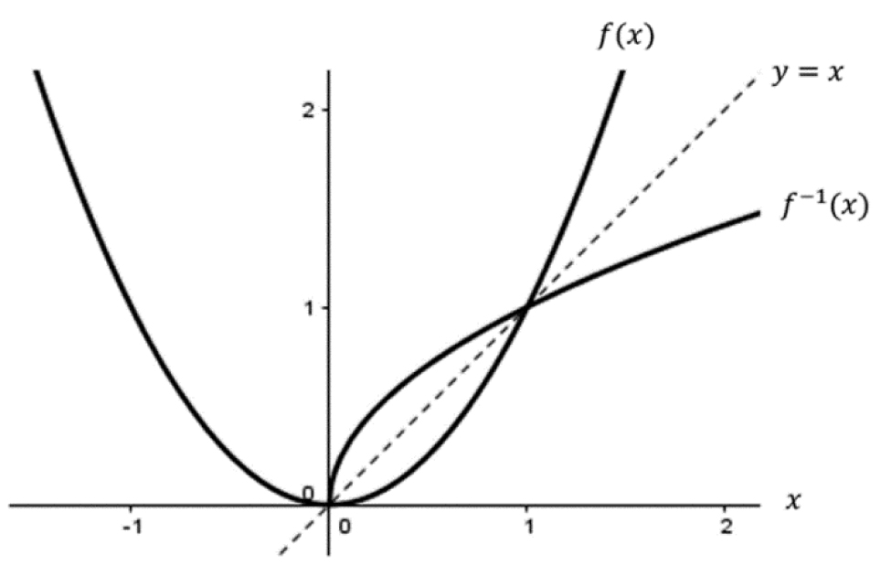
Figure 3.13. Graph of f(x) = x² and its inverse

The right side of the real plane looks correct, but what about the left side? Unsurprisingly, the outputs of f^–1 for x less than zero will live in the complex plane because the square root of a negative number will be imaginary. The mathematical blunder here is due to the fact f(x) = x² is not one-to-one on its domain.

Definition 3.7: A function is called one-to-one if every element in the range maps to exactly one element in the domain.

Since we could square the positive or negative version of a number and still get the same result, each of f′s outputs can be traced to two different inputs – violating the one-to-one condition. Therefore, f cannot have an inverse on its natural domain (all real numbers). We can use the horizontal line test to graphically determine if a function is one-to-one—which implies the function has an inverse. The general idea of the test is to imagine a horizontal line scanning the function from top to bottom. If the line hits the graph more than once anywhere, then f takes on the same value more than once—meaning each element in the range is not mapping to exactly one element in the domain. By applying the horizontal line test in Figure 3.14, we can conclude f does not have an inverse.

If a function fails the horizontal line test, hope is not lost. We can fix the issues with the domain by restricting it until the function passes the test. In our example, removing the left-hand branch and claiming the domain is x ≥ 0 will be enough to solve the problem. When we write the formula for the inverse, it is helpful to note the domain restriction. For example, f(x) = x² is 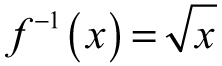for x ≥ 0 (domain restriction included).

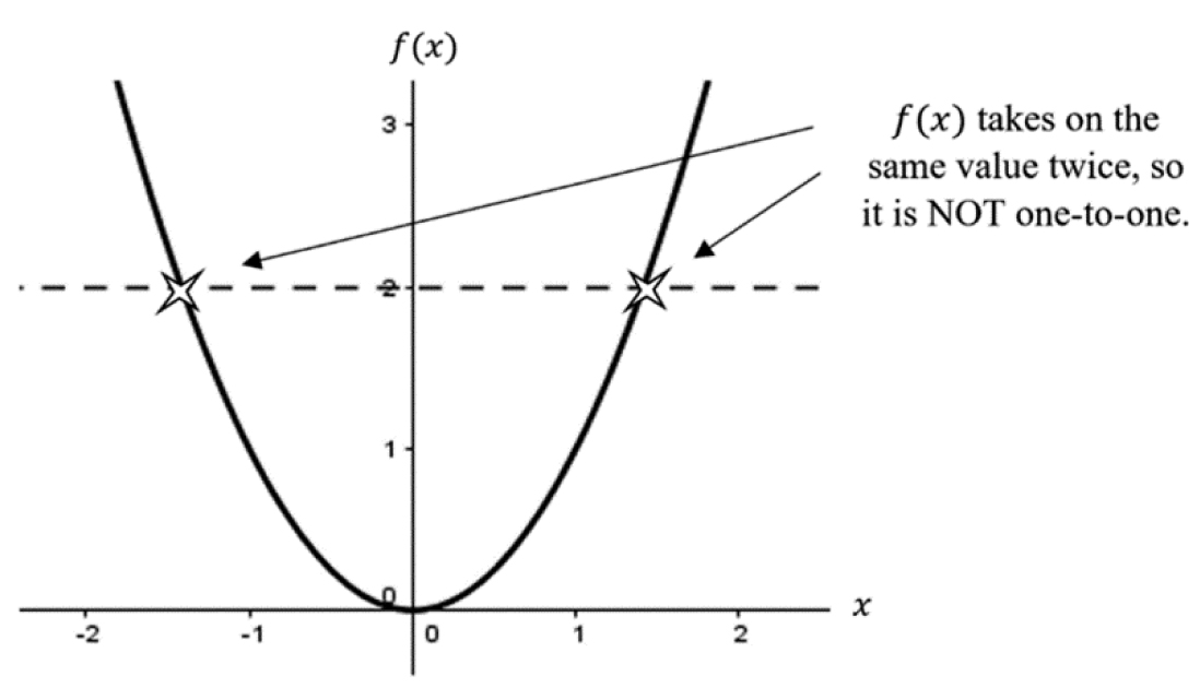
Figure 3.14. Demonstration of the horizontal line test

 

3.2 FITTING DATA

In practice, we often do not know what the entire function looks like; instead, we have a data set measured at different points (Figure 3.15). Although this may seem limiting, we have statistical tools at our disposal to interpolate and extrapolate.

 

Figure 3.15. A data set

Think about interpolation as playing connecting the dots; we make an educated guess as to how the x and y values are related. If there are enough data points, interpolation is safe to perform because there is usually sufficient information to make a reasonable prediction. On the other hand, we can consider extrapolation as the process of trying to connect the dots that are not even on the page. Given some data set, we attempt to guess what the data are going to look like before (or after) the point where we began (or stopped) making observations. If we only have a handful of points, this procedure is hardly meaningful—especially if we do not know what the function is supposed to look like. The distinction is further emphasized in Figure 3.16.

 

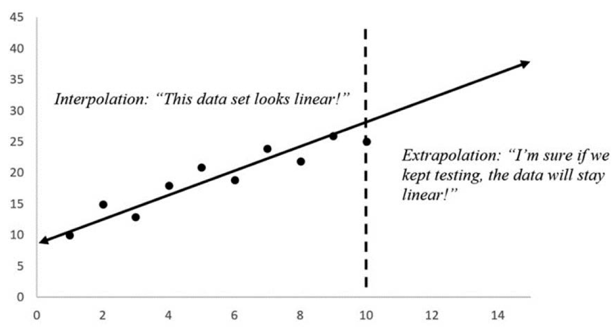
Figure 3.16. Interpolation versus extrapolation

We can guess what our function is going to look like by using the concept of curve fitting. This procedure can be incredibly useful in discovering or verifying laws we have come to embrace and use repeatedly in engineering. The type of curve fitting we will examine here is linear regression, finding a line that best fits the given data.

We often expect data to be linear within engineering, and when data are linear, we can find the best-fit line to show the best guess. Engineering students who may be anxious to have perfect results will sometimes “tweak” data, drop data points that do not “look good,” or otherwise manipulate their data to make it perfectly linear—this is generally unethical.

If something looks too good to be true, it usually is, and this includes measured data.

Example 3.8: Verifying Ohm’s Law—Fundamental in electrical engineering, Ohm’s law relates resistance (R), current (I), and voltage (V) through a simple linear relationship: V = IR.

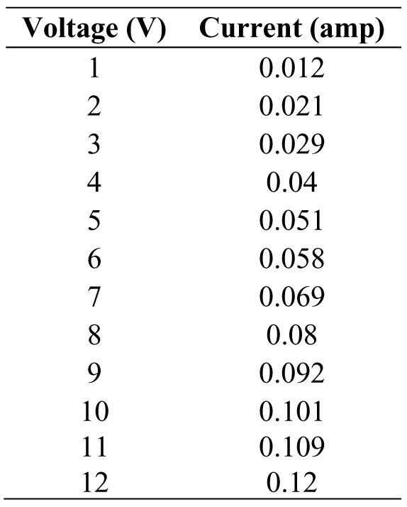
If we wanted to verify this law by going into a circuits lab, we could pick a resistor out of a box at random (say 100 ohms), turn on our power source, and let voltage drop over the resistor using the standard equipment. We measure the current flowing through the resistor in steps of 1 volt and end up with Table 3.4.

Table 3.4. Experimentally measured current for different voltages

Now, what do we do with this information? We would typically graph it, and to add meaning, we can use the method of least-squares fitting to find the best-fit line. To do so, we have to identify all of the important information to use the procedure.

First, how many observations were made? The number of samples or data points we collected is the sample size, denoted by N. When we measured the current, we made 12 observations, so N = 12. The variable we had control over was the voltage, so the independent variable is our collection of X values.

Definition 3.8: An independent variable is a variable whose values do not depend on another variable.

The current was our dependent variable because it depended on which voltage we set, so the current corresponds to the Y values.

Definition 3.9: A dependent variable is a variable whose values depend on another variable.

Next comes the tedious portion, calculating the following sets of data: XY and X², and adding up all of the columns individually (given by the Σ symbol). Why find XY and X²? Take a peek ahead in the formulas—just past Table 3.5.

Table 3.5. Calculating the necessary parameters for least-squares fitting

Now we can calculate the two parameters for the linear regression, the slope and the intercept. The formulas for the slope m and intercept b are as follows:

The linear fit (best-fit line) is L(x)= mx + b; this means our linear fit is L(x)= 0.0099x + 0.0006. Now that we demonstrated how to find this by hand, we can expose the dirty secret... this is usually done using a calculator, spreadsheet, or a program like MATLAB.

***

We found a fit! Now, how do we know we did well? If we plot the data set and the linear fit we found, the line narrowly misses almost all of the observations (Figure 3.17).

We can quickly figure out the degree to which the fit overestimates or underestimates the observations. Using this information, we can calculate the coefficient of determination (CoD), a quantity that measures how well a fit predicts the data.

 

Figure 3.17. Plot of linear fit from Example 3.8

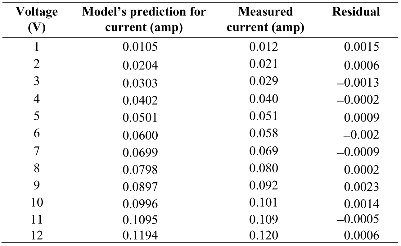
Example 3.9: Error in Fits, Residuals—We started with our original set, now we have a model for the data that can make predictions. This model—or fortune-telling function—we calculated as L(x) = 0.0099x + 0.0006, tells us what the current may be at each voltage. Let us evaluate L(x) at each of the voltages to see if the model gets close or not (Table 3.6).

Table 3.6. Table of predicted current versus the measured current

The natural next step is to check the difference between the model’s prediction and the measured value. For instance, when the voltage is 1 volt, then:

In the context of fitting data, this error is called a residual.

Definition 3.10: A residual is the error between a measured data value and the predicted value.

We can carry on and find the residuals for all of the data in Table 3.7.

Table 3.7. Calculating the residuals

In this case, the residuals are all quite small, which is to be expected due to the nature of the data. If we square the values in the residual column and add them up, we would have a sum of the residuals S_res (again, the Σ sign means “add up”).

If we know the average of the measured values and we subtract it from each of the measured values, we would have a sum of squares:

Then, the CoD we mentioned earlier is:

and can be calculated using Excel, MATLAB, or another similar platform. The closer the CoD is to 1, the better the fit! Considering Ohm’s Law is well known to be linear and we are performing linear regression, we do not expect much error in the amount of current we predicted versus the amount we measured. In this case, the CoD is 0.9988—an excellent fit!

Note that fitting data is an in-depth process and open to interpretation as to what constitutes a “good fit”—which is beyond the scope of this test. For best practices in this field, it would be wise to crack open a book on statistics.

***

 

3.3 LOCATING ROOTS OF A FUNCTION

An obsession in mathematics is finding roots of functions, or values of input(s) that give us a result of zero. Solutions to many problems in engineering depend on the idea of roots, so many methods exist to find them as a result.

In fact, one of the so-called Millennium Problems is concerned with finding roots to a particular function, the Riemann Zeta function, 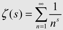, which is a bit outside the scope of this text.

Example 3.10: Finding Roots Analytically—Say we have a function modeling some velocity, f(x) = x² + 8x – 6, and we want to know what number or numbers make this function zero—which corresponds to the point(s) where the velocity is zero. The prescribed way to attack this problem is to use some sort of factoring method, but we cannot split it into factors no matter which numbers we try. This calls for completing the square. To begin, we set the function equal to zero:

Next, we force the left-hand side to factor by dividing the middle term by 2, so , squaring it, , or 16, and adding the result to both sides. This preserves the equality, even though it seems as though we are adding more numbers:

Do not be tempted to simplify this any further; we just brought out the number we needed to factor! Notice that the left-hand side, x² + 8x + 16, is a perfect square?

Now we can easily solve for x:

Therefore, either x = 0.6904 or x = –8.6904 will give us a value for f (x) = 0—this means the roots of this function are 0.6904 and –8.6904.

***

 

3.3.1 LOCATING ROOTS WITHIN A TOLERANCE, OR “GETTING CLOSE ENOUGH”

We did not need to use “completing the square” in order to solve the problem in Example 3.10, but it does provide insight into the ways in which we can play around with the expression in order to arrive at the solution. The most standard formula most of us know by heart is the quadratic formula, which enables us to find the exact roots to second-degree polynomials (quadratic equations). We know a quadratic equation, ax² + bx + c = 0 where a, b, and c are constants, has the following solutions:

This result is wonderful for equations involving x² terms, but can we solve equations like ax³ + bx² + cx + d = 0? Sure! We can solve third-degree equations exactly. Fourth degree too? Of course! Fifth degree? Well...sadly, no. Finding exact roots to a fifth-degree polynomial is just outside of our comfort zone. Although there are a handful of fifth-degree (or higher) equations that can be solved exactly, no universal formula exists. This means we need to settle for an approximation. One easy-to-grasp method we will explore is called the Bisection Method.

Example 3.11: Using the Bisection Method—Consider a function of the form f(x) = x⁷ + x⁵ – 1. The function, f(x), is a seventh-degree polynomial (since the highest power is a variable raised to the seventh power), which means attempting to find “exact” solutions will not be feasible options. Graphing the function in Figure 3.18 reveals there is definitely a root between 0.8 and 1, now it is a matter of approximating the solution. We will acknowledge there is a solution, x, which we will approximate iteratively using an alternate notation x^*.

 

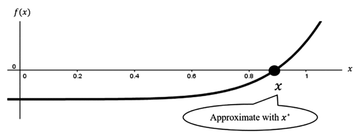
Figure 3.18. Graph of f(x) = x⁷ + x⁵ – 1 near the root

We begin by claiming our goal is to get as close to the statement f(x^*) = 0 as we can because finding the exact x such that f (x)= 0 may not be possible. Graphically, we deduced 0.8 < x^* < 1. How can we use this fact to our advantage? One subtlety to notice is that crossing the x-axis requires the outputs of f(x) to change signs; this is demonstrated in Figure 3.19. Anything below the x-axis is negative and anything above is positive.

 

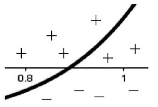
Figure 3.19. Noticing the change in sign around the root

To check, f (0.8) = –0.4626 and f (1)=1, so the sign did change! If we multiply these two quantities together, f (0.8) f (1) = –0.4626, the result is less than zero (negative). This is to be expected: if we multiply a negative number and a positive number together, we will get a negative answer each time. Let us generalize this to use as a root test.

Root Test: If we have an interval, [a,b], where a and b are real numbers, then there is a root in that interval if f (a) f (b)< 0.

Simple enough! The next question is how to proceed. In the spirit of the name “Bisection Method,” we are going to bisect the interval by dividing it into two equal parts. First, we will average the two end points and call it the first approximation, x^*₁:

Let us check to see how well this approximation does:

We are surprisingly close, but we can do better. Split the interval into two new intervals, [0.8,0.9] and [0.9,1]. Logically, we know one of these intervals definitely has the root, it cannot just disappear. How do we figure out which one though? Referring to our root test: if we have an interval [a,b], then there is a root in that interval if f (a) f (b)< 0. Let’s try it! For the first interval,

Ah, so the root is in the first interval. We can forget about the other interval then, we will only need the one containing the root. We us take the second approximation by averaging the two end points of the interval we kept and check how close we are:

Now we undershot the solution. We can continue by creating two more intervals as before, [0.8,0.85] and [0.85,0.9], and do the same root test. This process will continue until we reach some tolerance.

Definition 3.11: A tolerance is the acceptable error in a measurement or calculation.

To illustrate that we are making progress, Figure 3.20 provides a table with the attempt number, the estimated value of x^* found from averaging the end points, and the associated value of f(x^*). On the right-hand side, we have a plot of the attempt number versus the value of f(x^*). We can easily see the value of f(x^*) is gradually settling at zero as we make more approximations.

 

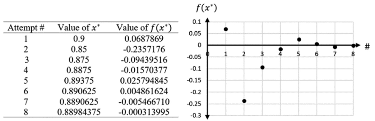
Figure 3.20. Table and plot of approximations from the bisection method

Where do we stop? Although there is an answer, we cannot find it exactly—so the approximations are our only hope. An easy tolerance to use is some extremely small number, ϵ. To check if we can stop, we take the absolute value of f(x^*) and look at the following inequality, |f(x^*)| < ɛ. The purpose of the inequality is to ensure we are “close enough” to the exact answer for the context of solving the problem. We can choose any small value we want, although there may be times where the problem statement (or real criteria) forces us to select a specific value for ϵ. For instance, say we want an approximation such that the output of f(x^*) is less than 0.001, so ϵ = 0.001—close enough, right? Under this tolerance, then the last attempt, number 8, will be sufficient.

***

Clearly only rough approximations should be done by hand. Choosing an extremely sensitive tolerance, such as ɛ = 0.000001, may require a large number of iterations to come close. To illustrate, Figure 3.21 showcases a tree-like diagram to illustrate how we calculated the approximation from the last example for the first three approximations:

 

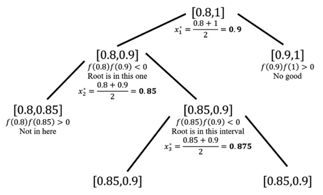
Figure 3.21. First three approximations of x^*

The moral of the story is to use technology for any extensive calculations like numerical analysis approximations. Engineers use computer programs like MATLAB to eliminate the long series of tedious steps we took in the previous example, especially with larger-scale problems. To summarize the method,

   1. Given a function, f(x), identify a point which is a root, claim you are approximating the root x by x^*, and enclose it with an interval [a,b] where a < x^* < b.

   2. Make an approximation 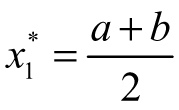, then form the intervals [a, x^*₁] and [x^*₁,b].

   3.Find the interval containing the root by testing if f(a)f(x^*₁) < 0 or f(x^*₁)f(b) < 0. Whichever one satisfies the inequality contains the root.

   4. Take the interval that satisfies the test and average the end points like step 2, this is the second approximation, x^*₁.

   5. Continue this process of breaking intervals in half and averaging end points until |f(x^*)| < ɛ for whatever tolerance ϵ is chosen.

 

Example 3.12: Approximation Techniques Using a Parameter—Some equations are plainly unsolvable, say we wanted to find an x such that:

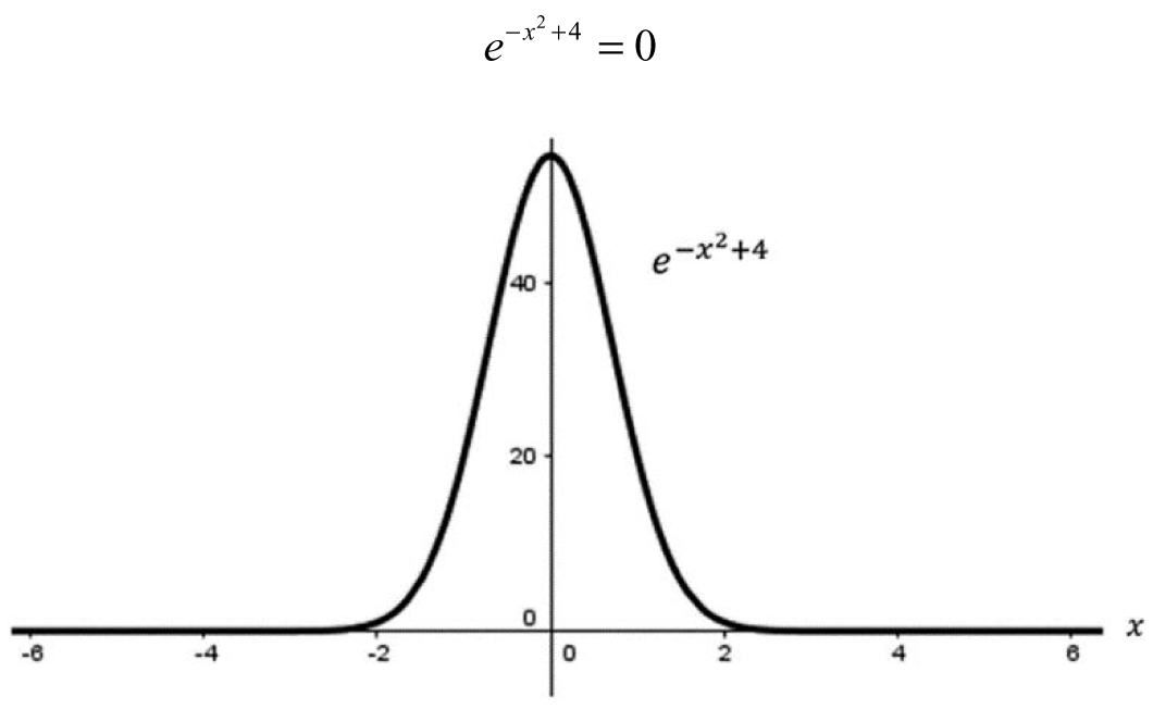
Figure 3.22. Graph of

In this case, we cannot find any solution because a number raised to a power can never be zero, despite what Figure 3.22 may lead you to believe (after all, it certainly looks like the function becomes zero as the value of x gets large in the positive or negative direction). We can get extremely close to zero, but never exactly zero. If we tried to solve this analytically using algebra, we would run into the following line:

which contains a mathematical “U-turn” sign, ln(0).

The natural logarithm of a number is represented by ln(x); this is the value of a number to which Euler’s Number, e, would need to be raised to such that it equals x. What is e? The number e is irrational, meaning it cannot be expressed as a fraction. It is defined as:

It may seem like an odd number, but it appears often in science and engineering.

What is 1n(0)? Well, phrase it a different way: “To what power do I need to raise the number e to in order for the result to be zero?” After thinking for a few moments, we realize no such number exists. However, we can get a general idea when the equation is close enough to zero—this is hinting at the idea of functional behavior. To do so, we introduce an extremely small number, ϵ, which is almost zero in this case. This number is called a parameter, and it transforms our problem that has no solution into one that has infinitely many solutions based on a number we are able to choose! To reiterate, ϵ is not an unknown, we have total freedom to choose its value. To demonstrate, we will solve the new equation:

This time, when we take the natural log of both sides, we would not get an error:

We were able to find two solutions! Not so fast though, our answer is now a function of ϵ, so we still need to test out some values for ϵ (Table 3.8).

Table 3.8. Values of the parameter and its associated value of x

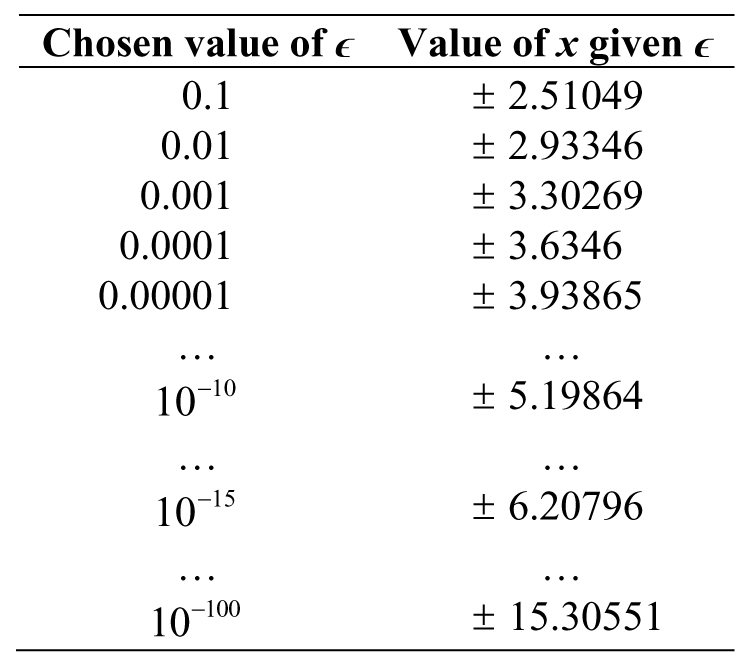
The question now is...which is the best answer? There are different ways of defining “best,” but let us say we are looking for the value of x where 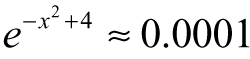; this would correspond to x = ±3.6346 since ɛ = 0.0001. The value of ϵ we chose could be called our tolerance or sensitivity as before.

***

 

3.4 FUNCTIONAL BEHAVIOR

As engineers, knowing the behavior of functions enables us to make extraordinary approximations and solve larger classes of problems. By behavior, we are referring in particular to the composition of the function, what the function does as it approaches certain values of interest, and what happens as the function takes on extreme values. Engineers like continuity in functions because it helps with the areas of interest we mentioned.

Definition 3.12: Continuity is a property in functions where sufficiently small changes in the input result in arbitrarily small changes in the output. If a function has this property, it is called continuous—otherwise, it is called discontinuous.

Intuitively, we view a function as continuous if we are able to draw the function without lifting our pen.

Example 3.13: Continuous Functions—The following functions can all be drawn without stopping and lifting our pens, so they are continuous. Figure 3.23 highlights a few examples.

 

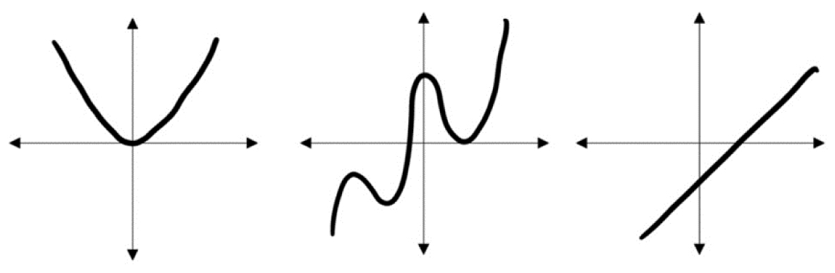
Figure 3.23. Continuous functions

Functions do not have to be continuous everywhere, they can have places where the function is discontinuous (Figure 3.24).

 

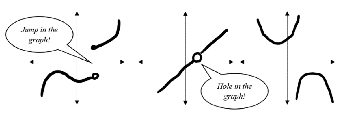
Figure 3.24. Discontinuous functions

***

All of the areas we are concerned with, values of interest, can be addressed through the implementation of a subtle operation called a limit.

Definition 3.13: A limit is the value that a function f(x) approaches as x approaches some value. Symbolically, 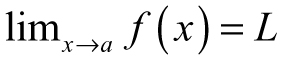means “the limit of f as x approaches a is L” where L is the limit.

Mathematically, the limit has a strict definition, but it is more practical to understand the limit as looking at a function through a different lens. In engineering, this operation of approaching values is not nearly as important as the concepts that use limits to formulate other arguments, but it can be useful to talk generally about the behavior of functions.

Example 3.14: Investigating Function Behavior—Suppose we have a function, , an important function in signal processing, and we want to look at some points of interest like x = 0. If we try plugging in x = 0, then we obtain the following headache:

Sadly, we cannot say much about this expression because we consider zero over zero to be indeterminate or undefined.

Definition 3.14: A function is indeterminate or undefined at some input if the output cannot be precisely determined (e.g., dividing by zero, infinity plus infinity, and so on).

This means f(x) has a “hole” at x = 0 and is discontinuous at that point; however, we can fix it. Take a look at the graph of f(x) in Figure 3.25.

 

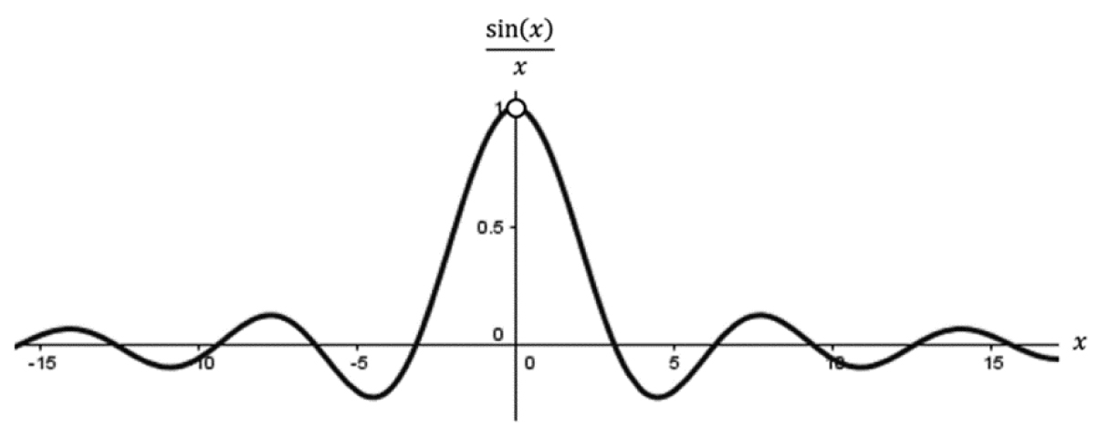
Figure 3.25. The graph of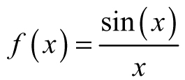

The hole where the result of f (0) should be can be repaired through a simple alteration; therefore, we can call this hole a removable discontinuity (in the sense we can “remove” the problem). The patch job is often done using limits; since f (0) is not defined, we will approach the point at x = 0 and see what we obtain (Table 3.9).

From our little investigation of approaching f(x) from both sides, we can see these values are approaching 1 from both sides (Figure 3.26). We might be tempted to say something like “Obviously, f (0) = 1,” but this is not technically correct in the mathematical sense.

Table 3.9. Approaching the value of x = 0

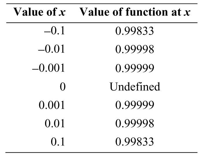
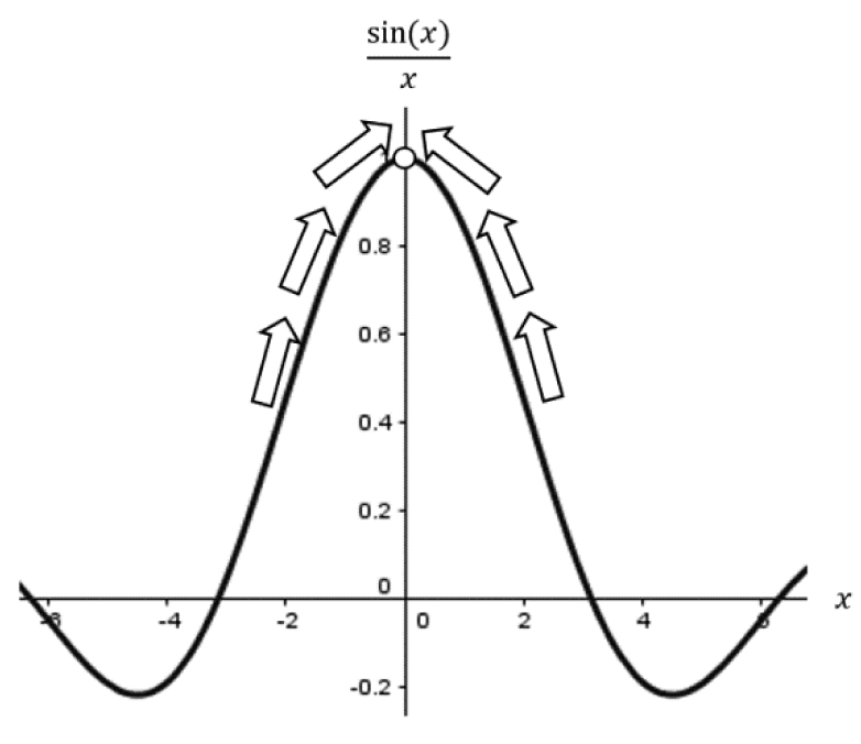
Figure 3.26. Limit approaching 1 from both sides

Instead, the limit of f(x) as x approaches 0 is 1...

With the limiting behavior, the function can redefined as sinc(x) – which is the exact same function we started with, but with the addition of the patchwork we did:

Discontinuity gone!

***

Functions can exhibit unusual behavior, most of which is influenced by particular values we put in place of x – these values are zeros and poles.

Example 3.15: Zeros and Poles—The most common functions to have a handful of these special values are rational functions, like:

A zero is just like a root; it is a value where the function is forced to zero. Since the function is a fraction, the whole function will be zero when the numerator is zero; therefore, we will set the top of the fraction equal to zero and solve for the appropriate values of x.

By factoring, we find the zeros are B2 and 2, nothing special. Through finding the zeros, we know where the function intersects the x-axis, which often has physical significance in engineering problems.

Poles are a bit more interesting, these hiccups in the function contribute to instability in systems if they occur in the wrong place. Instead of looking in the numerator, poles are values of the function where f(x) is not defined (i.e., where the denominator becomes zero). Setting the denominator equal to zero and solving:

The functional behavior for poles is best examined using limits. Again, we will approach the value from both sides and see if we are getting closer and closer to the same number. Let us check the pole at x = 4 (Table 3.10).

Table 3.10. Approaching the value x = 4

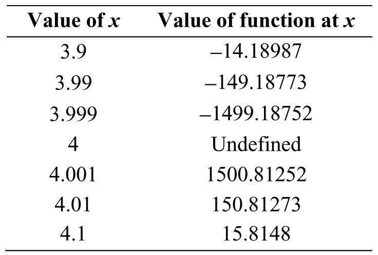
This time the function was completely bipolar. As we inched closer to the pole at x = 4 from the left, the values of the function plummeted; yet, the values of the function shot off upward when we approached from the right. In other words, the calculations are not approaching the same number from either side—which can be seen graphically (Figure 3.27). To be more precise, we can say that the one-sided limits do not agree. We take a one-sided limit by approaching a value of interest like we have been doing, but only in one direction (either left of the value or right of the value).To denote a one-sided limit and distinguish between the two, we denote the left-hand limit by saying “as x approaches 4^–” and the right-hand limit by saying “as x approaches 4⁺.” If the left-hand and right-hand limits do not agree, then the (regular) limit does not exist, “as x approaches 4.”

 

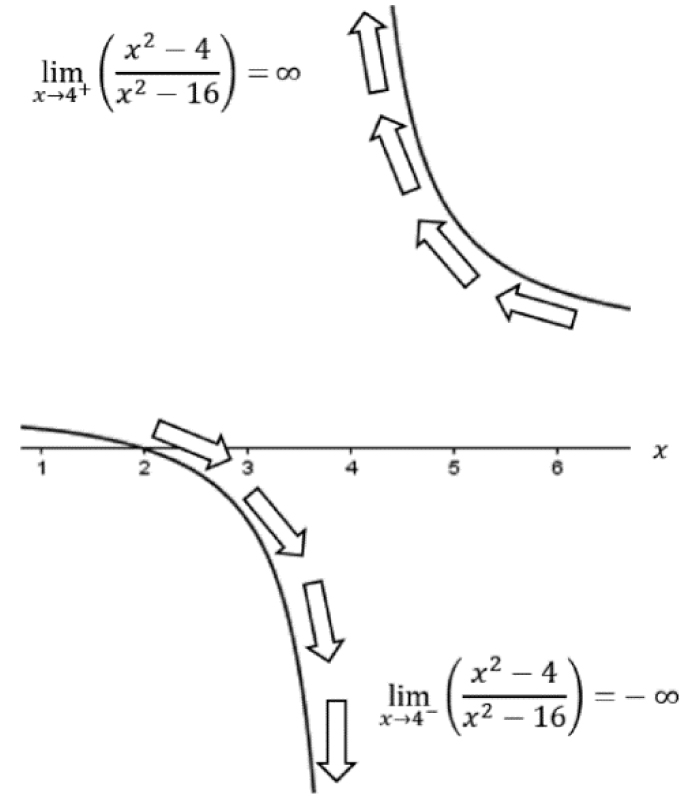
Figure 3.27. Disagreeing limits

The disagreeing limits provide us with more information if we plot the function around the value x = 4—we can see we have an asymptote. Put simply, an asymptote is an invisible line a curve approaches and comes ever so close to, but never touches. We know we have an asymptote if one limit is headed toward ∞ and the other is approaching –∞ or vice versa. A similar pattern can be seen if we checked around the other pole, x = –4.

***

Example 3.16: End Behavior—Another property of functions we are concerned with is what happens to a function f(x) at extreme values (large values of x, positive or negative) – known as end behavior. For instance, consider the function, f(x) = e^x, another superstar in mathematics, engineering, and nature in general. The limits to help us here and what they mean are

We will use the same method as before (Table 3.11).

Table 3.11. Approaching positive infinity

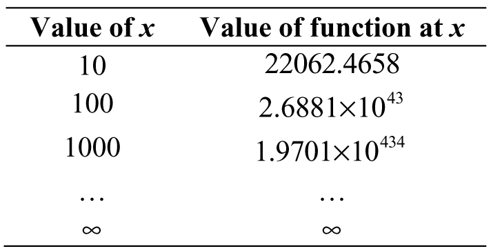
Even starting at x = 10 and increasing by multiples of ten, the value of f(x) is becoming so large, we needed to use scientific notation for x = 100. Without a doubt, this function increases without bound and approaches infinity:

Now, what happens on the other side of the real line, toward negative infinity? Using Table 3.12, we see a completely different trend.

Table 3.12. Approaching negative infinity

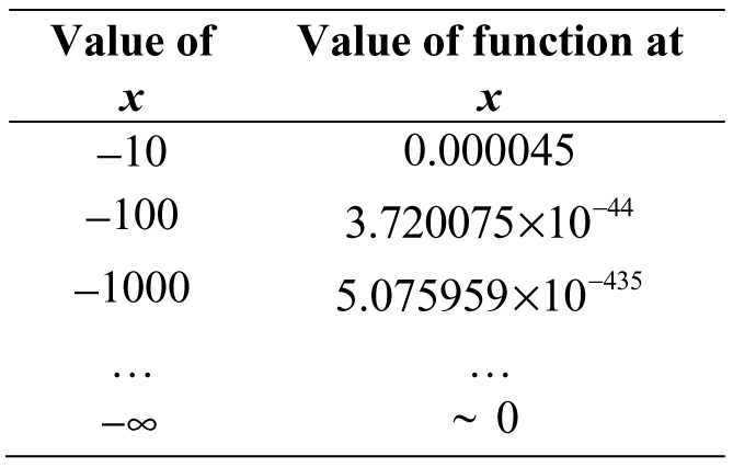
We still needed to dust off scientific notation to represent our results, but not for enormous numbers; instead, we needed to express numbers that kept getting smaller and smaller. If we continued Table 3.12, we would gradually start grazing the x-axis as the value of the function approached zero. Therefore,

Take care when interpreting this result! While the limit of this function as x approaches negative infinity (becomes large) is 0, there is no value of x where the expression becomes zero. Consulting the graph of f(x) = e^x in Figure 3.28, we can see our tables did not lie and our limits are correct.

 

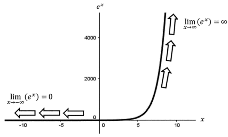
Figure 3.28. The function f(x) = e^x and its end behavior

***

Using the limit, we can define powerful new relationships between functions. Not only are we able to simplify functions, but we will also be eventually able to do some powerful approximations in the process.

Example 3.17: “Asymptotic to,” the Small-Angle Approximation—One motivating example prevalent in engineering is the calculation of the period of a pendulum. During the derivation, we arrive at the following expression:

where F is the sum of forces on the ball, m is the mass of the ball, g is the gravity constant, and θ is the angle the rope makes with the dotted reference line (Figure 3.29).

 

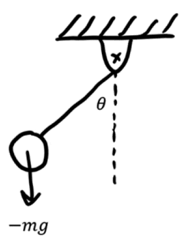
Figure 3.29. A simple pendulum

Our issue here is that we want to describe the motion of the pendulum primarily in terms of the angle, but the equation we would need to solve is fairly difficult (it happens to be a differential equation). To simplify the calculations, we consider what happens when the angle θ gets small. We can use the limit from Example 3.14 to help:

The limit above is a powerful result as it defines a so-called asymptotic relationship: “sin(θ) is asymptotic to θ as θ goes to zero,” which is written:

What is the physical meaning of this? To demonstrate, it is worth graphing both sin(θ) and θ in the same window as shown in Figure 3.30. The function sin(θ) acts exactly like θ for small values of θ! Therefore, we claim that sin(θ) is approximately equal to θ for this short interval—this is called the small-angle approximation.

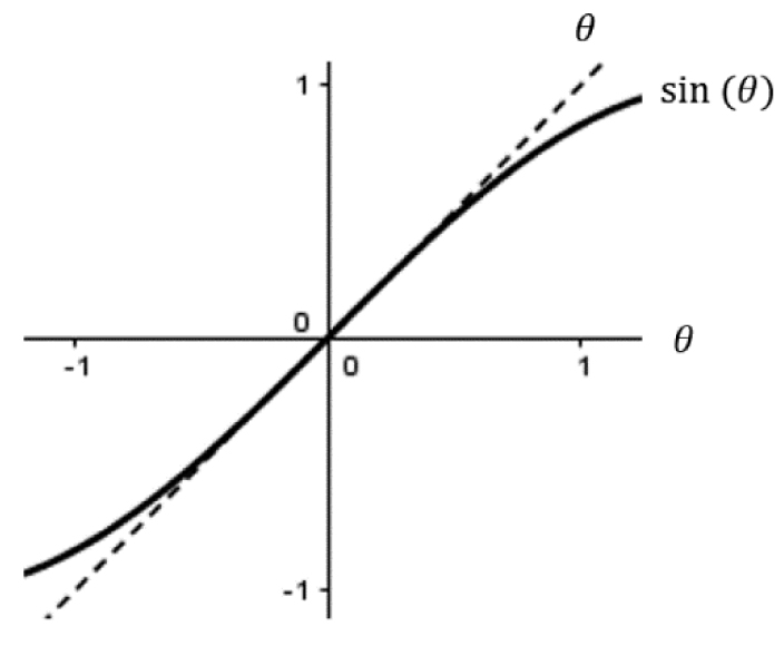
Figure 3.30. The small-angle approximation

Thus, our motivating problem reduces to

for sufficiently small θ, thereby reducing the difficulty significantly.

***

Example 3.18: “Negligible Compared With,” What is the difference?—When we examine functions at extreme values, it is likely some terms within a function will be less significant than others. For instance, consider the following two functions:

Suppose we wanted to examine their end behavior—what happens as the inputs head toward infinity? In other words, what are the following limits?

If we plug in bigger and bigger values for x, both functions will tend toward zero.

This can be seen graphically in Figure 3.31; however, there is another observation we can make. As we keep plugging in bigger values, the functions gradually melt into each other. This happens long before the inputs even reach triple digits!

 

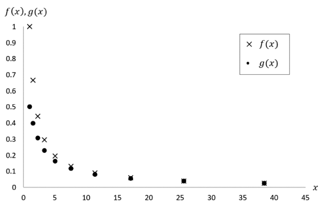
Figure 3.31. Comparison of f(x) and g(x)

This phenomenon is related to function behavior—the limits may be equal, but f(x) and g(x) are different functions. Despite this, we can reduce g(x) to f(x) using another subtle idea in engineering—“negligible compared with.” Like “asymptotic to,” we can use limits to understand what is happening. Let us isolate the denominator of the fractions: x and x + 1. As x gets bigger and bigger, the value of x gradually dominates the 1, making the 1’s contribution less noticeable. In terms of a limit,

or in words, “1 is negligible compared with x, as x goes to infinity.” We can then say:

We might be tempted to jump one step further and claim that g(x) = f (x) for large enough x, but that is not technically true—even though they look extremely close on a graph, they are still separate at each point (although their difference might be infinitesimally small).

***

To use these operations in practice, we need two functions f(x) and g(x) and a point of interest, some number we will call a (which could be infinity). Then,

and

Note that g(x) cannot be zero in both definitions, otherwise we would be dividing by zero (clearly not smart, or even mathematically legal).